Chux's Notebook
This is a collection of my notes which I refer to on a regular basis. Hope it is also helpful for others stumbling by.
I think of these notes as mountaineering pegs. Often at the time of studying a particular paper or topic, the concepts are clear. Over time, however, only a vague impression remains, and I can no longer tussle with the issues. So these notes serve as pegs that I hope to use to re-scale an old hill, or at least scale it with less effort than starting from scratch.
Generally, I highlight main points like so, and put in-line code or numbers like so.
Built with mdBook.
About Me
I am working as a Lead Data Scientist at GovTech Singapore, on a team called JumpStart. We power search and recommender systems for Singapore Government products like the job searching portal MyCareersFuture or the CareersFinder tool to discover next steps for one's career.
My LinkedIn profile is here.
Current Focus
2025 Goals
Incorporate semantic IDs into a generalizable search and recommender system:
- Can function well with just a system prompt (guiding the overall goal of the system) and an item catalogue
- Handles a changing catalogue gracefully
- Good search and recommendation latency
- Cheap (runs on a T4 or equivalent)
Research Questions
-
Optimizing LLM explanations based on implicit feedback
- How to optimize an LLM to provide better recommendation explanations by fine-tuning on implicit feedback?
-
Replacing BM25
- How to design a search system that matches BM25 performance at cold start and gradually improves with more data, without dropping below BM25 performance?
-
Precise Retrieval
- The common two tower approach to embedding retrieval leaves much to be desired
- There is no natural score threshold at which items are deemed irrelevant. Traditionally, classifiers have a
0.5score cut-off. - Embedding retrieval tends to retrieve unrelated items. This is a well documented problem. For example,
Nike shoesretrievesAdidas Shoes. - Can we have embedding models that approximate AND / OR conditions that more naturally fit into the retrieval paradigm?
- There is no natural score threshold at which items are deemed irrelevant. Traditionally, classifiers have a
- The common two tower approach to embedding retrieval leaves much to be desired
-
Efficient learning of semantic IDs
- LLMs can learn Semantic IDs as part of their language and recommend and reason about items once they learn the "language" using Supervised Fine Tuning
- But the danger is catastrophic forgetting and losing capabilities as they get fine tuned in this way
- Is there a more "natural" way for LLMs to learn such semantic IDs?
- How do we handle a changing catalogue in real-time gracefully?
Thoughts
Short notes and ideas.
On ML Experiments
On using LLMs (e.g. Claude Code) to assist with ML experiments, especially on replicating existing results from papers.
There is much value in replicating ML experiment results from papers.
- Forces one to understand and implement the methods in the paper, no shortcuts
- Helps one understand how sensitive the results are to hyperparameters, data settings etc.
- Allows one to test out new methods or variations on the same task for an apples-to-apples comparison
Traditionally, this takes some time for each paper (days to weeks) depending on the complexity of the method, the compute cost, the expertise of the researcher who is performing the replication etc. There is also significant ambiguity in what defines a successful replication, since the paper may have inadvertently left out some implementation details, and the results might not be exactly replicable.
LLMs can make this process a lot faster, by:
- Performing requisite data cleaning
- Implementing the methods
- Monitoring the training and validation runs and fixing bugs along the way
This raises the question: what are the respective roles of the LLM and researcher in such a process? From my experience, I have tested out these loosely described paradigms:
- Iterative LLM-assisted coding
- Basically not too different from development before LLMs - the researcher codes from scratch and gets LLM to assist with each function, testing small pieces as we go along
- Spec-driven LLM development + post-hoc checking
- Researcher starts with detailed specifications file, detailing as much as possible about the data, method, hyperparameters, implementation process, evaluation criteria etc.
- LLM implements semi-autonomously, checking against the specifications
- After each phase, researcher reviews the code to understand it, refactor it, simplify it etc.
- Fully autonomous LLM
- Researcher provides the full paper to the LLM and high level specifications
- LLM implements end to end and submits results
I find that approach 1 produces the cleanest repo and understanding for the researcher. But it is also the slowest - significant time is spent debugging and doing the code edit -> run code loop manually. It's probably the approach that most researchers are using currently, to varying degrees of autonomy given to the LLM.
I could not get approach 3 to work. I tried running Claude Code in --dangerously-allow-permissions mode on runpod, and give it almost full autonomy in implementing and running the code. Some frustrating points:
- LLM kept using synthetic data even for the full run, even when explicitly spelled out that synthetic data is only for dev runs. When asked why it was using synthetic data, it said it failed to download the data. But managed to download the data on the very next instruction.
- LLM has no common sense. The paper detailed its method of generating synthetic queries on movielens using an LLM (since movielens only has interaction data) to train a search biencoder. Claude decided to generate synthetic queries of the form "What movie is
<title>?", despite being told to use an LLM to generate from the movie text. Such hard-coded queries obviously led to very high accuracies of> 99%, but Claude did not know to terminate and investigate. - LLM did not create meaningful evals. It mostly monitored train and validation loss, and even these were not very meaningful (it decided to sample only
500points for validation). The researcher needs to be explicit about specifying these.
Some reflections on testing out approach 3:
- Verification is hard in ML tasks. I tried providing the accuracy results from the paper to the LLM, asking it to benchmark against those figures to see if it is on the right track. The LLM was way off but did not know how to troubleshoot such problems. Normal test driven development also does not work for ML Tasks.
- Difficult to debug in fully autonomous setting. ML tasks are very sensitive to how the data is processed, hyperparameters etc. Even a small decision like left or right padding can significantly change results. Without diving into the code, I had no means of forming hypotheses about what was messing up the performance. LLMs are not well trained in this task of playing detective, and interrogating it did not yield much fruit.
- Unpleasant to understand code. Giving LLM full autonomy produces a lot of code that is intimidating to try to grok. I can probably do it with LLM assistance, but it produces the same daunting feeling as reviewing a large pull request. It also feels like unnecessary work as it entails spending time trying to understand lots of glue code.
Which leads me to approach 2. This is the approach I am currently testing out. The hope is that spec-driven development is a good middle ground. The researcher gets to use the specification to determine how far we want the LLM to sprint in each run, before we apply manual verification and understanding. This minimizes the chance of LLMs running completely off point and also makes it more palatable to understand a small piece of code each time.
Front-loading the development of specifications also forces the researcher to adopt systems-level thinking and design for the whole experiment. This hopefully helps us move up a level of abstraction and move along faster.
The main difficulties of approach 2 a-priori to me are:
- Designing the right places to pause for manual verification and understanding
- Getting the LLM to follow our specs closely and stop at the correct checkpoints
Will test it out and see how it goes!
On AI Assistants
The popularity of Openclaw and its variants show that there is much interest and fascination with having a personal AI assistant to make us more productive etc. However, after thinking about it for some time, it seems not so trivial in designing an AI assistant that actually helps (vs appearing to help).
I think my desiderata for a helpful AI assistant (in roughly descending order of importance) are:
- Reliable. Able to autonomously and reliably complete non-trivial tasks (e.g. tasks that normally take a few hours of my time)
- No brain rot. Do not replace or shortchange my own grokking process as a result of said offloading
- Self-learning. Able to learn and improve over time based on my interactions with it
- Tool access. Able to read/write/act on local data files or permissions to apps that I pass to it
- Accessible. I am able to communicate (both input / output wise) with the assistant via convenient means (e.g. slack, telegram etc.)
Vanilla chat-based UI LLMs fulfil (1) reliable and (5) accessible. However, their self-learning and tool access are limited.
I think these are the main pros of openclaw and its variants - the promise of (3) self-learning, creating its own tools, persisting these in a local environment, and (4) extensive permissions to interact with our files and applications (e.g. calendar, email etc.).
These are also the easier problems to solve. The hard problems are in (1) reliable and (2) no brain rot, for which I elaborate some thoughts below.
"Reliable" is task dependent
I think the main killer of AI assistant usage is reliability for the specific tasks that people are interested in. AI assistant reliability has passed the [for info] benchmark but is often not sufficient at the [for action] level.
For example, it is not straightforward to use AI assistants to run ML experiments. I'm trying to find the best harness for doing so (when I have time), but naively using claude code has resulted in pretty bad outcomes for me. For example, it insisted on using synthetic data instead of downloading movielens as per the paper I assigned to it - I only discovered this when the validation accuracies were abnormally high.
The problem of reliability is related to the "brain rot tax" (see below). When I am doing my own research, I gain an internal mental map as I go along that allows me to auto-correct wrong things I encounter along the way. With LLM-generated output, it feels like all-or-nothing - either we are able to trust the output 99% or we are not able to trust it at all. Suppose 80% of the report is gold and 20% is dross. We do not have the mental tools to correct the 20% because we don't know which 20% is the dross.
Another way to say a similar thing is to call it a "verification tax". Unless we have strong apriori evidence or experience to trust the output, we will have to either spend effort verifying the reliability of the output or live with a nagging feeling that something could be very wrong somewhere. The effort spent to verify the output could have been better invested in doing the research ourselves instead.
Again, my sense is that the relationship of LLM usefulness to reliability is not linear - meaning that reliability of 79% does not make it doubly useful than reliability of 40%. Instead, I think usefulness is near zero at low levels of reliability, and there is a threshold at which utility shoots up. It then grows exponentially as reliability approaches 100% before tailing off. A system that is 90% reliable is way more useful than 80%, and 95% way more than 90%.
There is a chicken and egg problem in that we need to be an expert to design and evaluate an LLM system to have high reliability, but we often need LLM systems in areas that we are not experts. Hence the verification tax is very high for such greenfield areas that are also the most useful.
The "brain rot" tax
Criteria 2 (no brain rot) is somewhat categorically distinct from the others, because it is not so much the tool itself but how we use it that can result in brain rot. However, I think it is worth a mention, because to me it is one of the main factors hindering effective use of AI assistants, especially for knowledge tasks.
There is a viral post going around about tool-shaped objects that hits on this. The danger is that we often subconsciously equate lots of LLM activity with lots of productive work being done. However, this is only true if the output of the LLM activity is all we need, and the journey of getting there can be safely discarded. In reality, the journey of getting there for many knowledge tasks is just as important, and discarding the journey greatly reduces the value of the whole undertaking.
Take a research task for example. Suppose my goal is to deeply understand a particular subject. I instruct an LLM to generate a deep research report about said subject. The value of the report will not be realized until I start reading and interacting with it, asking questions, probing and trying to align my mental model with what is presented. All these activities are not captured in the report itself - they stem from my own initiative. Thus it is hard to design an AI assistant that will automatically ensure grokking happens without the user being very intentional about how they use the outputs.
Furthermore, it is not obvious apriori what form of interface best facilitates grokking, and it also varies by person and by task per person.
Thus it seems that there is always some brain rot "tax" of trading output against understanding when we use LLMs for knowledge tasks. We either recover the "tax" by separately engaging the material in intentional ways, or absorb the tax and just focus on using the output for whatever downstream purposes. Either way, there is a cognition tax that takes away from the benefits of LLM output, and often it becomes a wash.
There is probably value in designing AI assistant interfaces that explicitly mitigate brain rot through various mechanisms, such as testing the user. But I have not seen much of this yet. My own code-stories is a small attempt to find ways of encouraging user understanding of LLM material.
Conclusion
There is no clear way forward currently. My sense is that we have to be intentional in designing specific sub-agents for each task that we want the AI assistant to do, and think carefully about the input / output medium to give us confidence that it is (1) reliable and also discourage (2) brain rot. The openclaw agent is more of an orchestrator to glue things together, but the default chat interface is not ideal for many high value tasks.
On Research Flow
Work-in-progress thoughts on how to design a personal research flow.
Paper Reading
Paper reading can be split into 4 levels:
- Skim. Read AI-generated summaries based on a structured prompt to decide whether a paper is worth a close read. Sections may include:
- Main Contribution
- Main Competitors
- Ablation Studies
- Main Limitations
- Medium Dive. Use a CodeStories-like approach to generate an AI deep dive which is easy to browse on-the-go but still offers depth
- Deep Dive. Writeup about the paper on this blog, possibly referencing the medium dive material. Go deep into the equations and math.
- Replicate. Replicate the method and reproduce the results of the paper. This falls partially under experimentation flow .
Realistically, the quantity of papers under each category will be funnel-like:
- Skim: almost every paper in my field of interest
- Medium Dive: almost every major paper (definition of major TBD)
- Deep Dive: major papers on the topic that I am actively researching
- Replicate: subset of deep dive papers
So I need a paper reading flow like that:
- An automated discovery pipeline for finding papers to skim
- Possibly using picoclaw, or setup a more principled approach designing something around
claude -p - Allow manual addition of papers that I encounter
- Allow steering of paper discovery process (more like this, less like this)
- All papers should automatically go into my dropbox
- Possibly using picoclaw, or setup a more principled approach designing something around
- A process for assigning papers for medium dive
- Probably using picoclaw + a PaperStories interface is sufficient
- Expose the story on laptop + phone for browsing
- TBD possibly a testing interface to make sure I understand
- Deep dive is on my discretion, no workflow needed here
- Replicate requires a good experimentation workflow, covered in another section
Experimentation
More thoughts on experimentation next time. How to:
- Steer an agent to write experimentation code
- A good medium to read the code and give comments for refining
- Effective debug / full run on correct hardware (local CPU? local GPU? modal?)
Requirement: effective experimentation should be >90% steerable via conversation. But details / observability matter a lot for ML experiments.
Recent Trends in Search & Recommendations
This document summarizes some important ideas in both recommender systems and search systems that have emerged in the past few years. It aims to be a helpful read for someone trying to get acquainted with modern practices in these fields.
What we will cover:
- Embedding learning. Embedding learning for items and users is an upstream task that are used for downstream retrieval and ranking.
- Recommendations
- Search retrieval and ranking
Embedding Learning
Embedding learning is a foundational tool that powers all recommendation and search systems. Typically, users and items are represented by one or more embeddings that get fed into neural networks for prediction and recommendation tasks.
Whilst many off-the-shelf LLM embedding models exist today, the best performing embeddings are often context-specific. For example, from the perspective of a job-seeker, we may want the embeddings for Physical Education Teacher and Gym Trainer to be similar, as the focus is on similar job functions / skills. However, from the perspective of a HR personnel trying to do manpower planning, we may want Physical Education Teacher to be more similar to Executive at Singapore Sports School, since the focus is more on eligible pathways for internal rotation (btw, I made this example up). Hence, there is a need to effectively learn embedding models in a specific product setting. Lee 2020 describes the task like so:
(the goal is to) Learn embeddings that preserve the item-to-item similarities in a specific product context.
It is common practice to have an upstream pipeline to learn item embeddings that get re-used for multiple downstream tasks (let's call this a "universal" embedding). For example, YouTube uses a common set of video embeddings used by all its models [Lee 2020]. To adapt the embeddings to a specific task, the task model itself can always add a simple translation MLP layer to translate the universal embedding so that the embeddings can be more performant in each task setting.
Another way is to have each retrieval and ranker model learn its own embeddings for its specific task.
- However, this leads to redundancy to store and update each set of embeddings, often in some in-memory feature store, which is costly.
- This approach is also often not as performant as learning a universal set of embeddings and then adapting the embeddings to each task via a small learned MLP layer
- Training from a frozen set of universal embeddings is also much more compute efficient, as we do not need to forward/backward propagate into a potentially large language model that generates the embeddings from text or some other modality.
We can think of upstream training of an embedding model as analogous to the common practice of pre-training large language models in a semi-supervised manner on a large text corpus. The LLM is then fine-tuned for specific applications.
Although the performance of using multiple embeddings to represent an item has been proven to be more performant than using a single embedding (e.g. using ColBert), most companies seem to adopt a single embedding to reduce engineering complexity. For example, Pinterest briefly experimented with multiple embeddings per item but reverted to a single embedding to reduce costs.
There are 3 primary ways of embedding representation in the literature:
- ID-Based: This method maps an item's ID directly to an embedding.
- This is often used in a task-specific model, but not usually used for a universal embedding model shared by downstream tasks, as we cannot represent new items that have no user activity
- Content-Based: This is the most common approach, generating embeddings from an item's content, such as its text, images, or audio
- Textual content is usually passed into an LLM to generate embeddings
- For other modalities, task-agnostic preprocessing may be employed. For example, Lee 2020 sampling frames from a video and runs them through a ResNET model to create raw embeddings before they are fed into the main embedder model
- Graph-Based: This method can be seen as an extension of the content-based approach. It generates an embedding from the attributes of an item's neighbors in a network.
- This is particularly effective in social network products where network interactions are crucial, such as on LinkedIn, Pinterest, or Facebook
- While powerful, this method is more computationally expensive at both training and inference times because it requires access to the graph to compute embeddings
Embeddings are typically trained in a contrastive learning manner, which simply means that we want to encourage related items (e.g. videos frequently co-watched) to have high similarity scores and unrelated items (e.g. randomly sampled vidoe pairs) to have low scores.
Thus, we can think of contrastive learning as comprising 3 main components:
- Positive Sampling. How we mine for related items from data is a non-trivial, but an oft-neglected topic. Usually some behavioural statistics are used, e.g. Lee 2020 uses
videos frequently co-watched by usersto determine positive pairs. The guiding principle is to err on the side of being stricter in the selection of positive samples to minimize the appearance of false positives in the data (which are more harmful than false negatives).- In JumpStart, we have explored using Pointwise Mutual Information score to discard item pairs with low PMI score. Recall that the PMI score is computed as:
- Considering co-occurrence statistics focuses only on the numerator. Normalizing by the marginal probabilities of the items reduces the incidence of popular items being labelled as related when they are actually not
- In my experience, the bottom
10%of co-interacted items by pmi score can be safely discarded - Another subtle issue is that power users contribute disproportionately to positive pairs.
- If a given user interacts with items, then he/she generates item co-occurrence pairs
- The quadratic scaling in means that the item interactions from power users may dominate that of all other users, but these are also the least informative item pairs :'( as power users may have less specific item preferences
- Hence it is advisable to discard power users beyond a particular percentile to improve positive sampling
- Negative Sampling. Much of the research literature focuses on this issue. The reason is that as research data (e.g.
Movielens) is fixed, the positive pairs are usually pre-determined in the data. But the negative samples are usually not pre-specified in the data, so methods are devised to sample:- Random sampling. This is the simplest and most common approach: for a given anchor item, we sample negatives uniformly from the item catalogue, omitting the positive item(s) for the anchor
- Impressed but not positive. This is also a simple approach if we have access to item impression data. The impressed items are often hard negatives because they were deemed to be relevant by the existing recommendation system and surfaced to the user.
- The potential danger is that the model may only learn to distinguish negatives in a specific retrieval setting and is not robust to changes in the retrieval model
- Hard negative mining. Various other methods exist to mine for hard negatives, e.g. using BM25 score or embedding similarity. We discuss two ideas on this below in a bit more detail.
- Usually, it is best to mix negatives from all of the above so that the model learns to distinguish positives from a wide range of negatives
- Loss. Again, much ink has been spilt on this topic, but there are really only two main losses that we need to know:
- Triplet loss.
- Cross entropy (or InfoNCE) loss.
WORK IN PROGRESS
To improve training, two ideas are critical:
- Semi-hard Negative Mining: Originating from FaceNET, this technique addresses the problem of "false negatives" (items that are incorrectly labeled as negative) which can confuse the model. It focuses on training examples that are in a "goldilocks zone"—not too easy and not too hard. Lee (2020) demonstrated that mining for the hardest semi-hard negatives within a mini-batch is a computationally cheap and critical step for model performance.
- Smart Negative Sampling: Since random sampling often fails to find challenging negative examples, methods are devised to mine for them. This can involve using impression data, surrogate algorithms like BM25, or approximate-nearest-neighbor search. Lee (2020) also introduced using hierarchical clustering on a relational graph to find negatives from nearby clusters, which can be combined with semi-hard negative mining to prevent issues with false negatives.
From Matrix Factorization to Sequential Recommendations
Traditional matrix factorization methods learn a single, static user representation to predict their entire interaction history. This is problematic for users with diverse or evolving interests, as the model learns a "diluted" representation. While time-decayed ratings can help by giving more weight to recent interactions, the model still fails to learn the sequential nature of those interactions fully.
Sequential recommenders address this by mirroring the actual recommendation task: given a user's history up to time t, predict their next action at time t+1. The user's representation is therefore dynamic and based on their recent actions. There are three main approaches to this:
- Markov Approach: A simple but often effective method that uses the last interacted item as the primary feature to predict the next one.
- Pointwise Approach: This method involves "rolling back" features to what was available at the time of each action in the training data. While this explicitly computes every user-item interaction, it requires significant data-loading effort and careful feature engineering. Google chose this approach for its simplicity in distributed model training.
- Sequential Modelling Approach: This is analogous to language modeling, where the model learns to predict the next item in a sequence, learning from many items simultaneously.
Case Studies in Sequential Recommendations
Covington (2016) - Pointwise Approach at YouTube:
YouTube's influential 2016 paper detailed a pointwise approach for both retrieval and ranking.
- Retrieval: The model used features like the average embedding of the last 50 video watches and search queries, along with user features like gender. A small MLP was trained with a sampled softmax loss to predict the next video watch. A crucial finding was that predicting the next watch was far more effective in online A/B tests than predicting a randomly held-out watch from the user's history.
[Diagram: Pointwise Approach for Retrieval - Covington 2016 architecture from slide 13]
- "Example Age" Feature: To capture the time-sensitive nature of video popularity, an "Example Age" feature was introduced. This simple feature encodes when an action took place, allowing the model to learn the "popularity lifecycle" of items, where popularity often spikes shortly after upload and then fades.
[Diagram: Chart showing Class Probability vs. Days Since Upload with and without the "Example Age" feature, from slide 15]
- Ranking: The ranking model was similar to the retrieval model but incorporated many more features, particularly those related to user-item historical interactions (e.g., "how many videos from this channel has the user watched?"). The paper noted that even simple transformations of features, like square roots, improved performance, highlighting the reality of manual feature engineering.
[Diagram: Pointwise Approach for Ranking - Covington 2016 architecture from slide 16]
SASRec (2018) - The Transformer-Based Approach:
SASRec (Self-Attentive Sequential Recommendation) applied the transformer architecture to recommendations, treating a user's interaction history as a sequence of items to be predicted, much like words in a sentence.
- Architecture: Using causal masking, the transformer embedding at each time step encodes all previous interactions. The training loss is typically a binary cross-entropy loss comparing the dot product of the model's prediction with the target item embedding against a random negative sample. This approach significantly outperforms traditional matrix factorization methods.
- Position Embeddings: Since transformers have no inherent notion of sequence, SASRec adds a learned position embedding to each item in the input sequence. This helps the model weigh recent items more heavily, as shown by visualizations of the attention matrix.
- Efficiency and Power: This paradigm is more efficient than the pointwise approach because it learns from N time steps simultaneously for each user. It also reduces the need for manual feature engineering, as the model can implicitly learn user-item interaction features.
[Diagram: Visualization of Average Attention Matrix from SASRec, with and without Positional Embeddings, from slide 21]
A subsequent paper, BERT4Rec (2019), proposed a "masked token prediction" task similar to BERT, allowing the model to use future items as input. While it initially appeared superior, Klenitskiy (2023) showed this was due to a difference in loss functions; when both use the same sampled softmax loss, SASRec consistently performs better and trains faster. The conclusion is that SASRec with sampled softmax loss is the current industry standard.
PinnerFormer (2022) - Long-Term Sequential Modeling at Pinterest:
PinnerFormer evolved from the need to switch from real-time user embedding computation to less costly daily batch jobs.
- Long-Term Loss: The key idea is that at each time step, instead of only predicting the very next item (like SASRec), the model predicts a random item from the user's future interactions over a longer window (e.g., 28 days). This creates more stable embeddings and surprisingly, PinnerFormer beats SASRec even when retrained in real-time.
- Advanced Features: PinnerFormer uses pre-computed PinSage (graph-based) embeddings as a base. It distinguishes between different action types (e.g., "Pin Save" vs. "Long Click") by concatenating a learned "action" embedding to the item embedding. It also heavily relies on time features, using Time2Vec to encode timestamps, noting a significant performance drop without them.
- Training Details: The model uses a combination of in-batch and random negatives with Log-Q correction, and ensures each user in a mini-batch is weighted equally to avoid bias from users with very long histories.
[Diagram: Illustration of PinnerFormer's "Long Term Loss" compared to SASRec from slide 25]
Multi-Task Learning in Recommendations
Recommendation systems often need to optimize for multiple objectives (e.g., clicks, saves, purchases). Several architectures address this, primarily for the pointwise approach:
- ESMM (2018): This model explicitly encodes the relationship that a conversion can only happen after a click (
P(convert) = P(click) * P(convert|click)). This allows the conversion model to benefit from the abundant click data while learning from the sparse conversion data.
[Diagram: ESMM architecture from slide 29]
- Shared-Bottom Architecture: A common approach where bottom layers of a neural network are shared across tasks, with separate "towers" or heads for each specific task prediction. The final recommendation is a manually tuned weighted average of the logits from each head.
[Diagram: Shared-Bottom Model architecture from slide 30]
- Mixture of Experts (MoE): An improvement over the shared-bottom model, MoE uses specialized "expert" layers. For each task, a gating network learns a weighted average over the outputs of these experts, allowing the model to modularize and handle potentially conflicting tasks more effectively.
[Diagram: Multi-gate Mixture-of-Expert (MoE) model architecture from slide 31]
- PinnerFormer's Approach: For sequential models, PinnerFormer took a simpler route, finding that treating all positive actions (repins, clicks, etc.) as equal signals was the best all-around strategy for their use case.
| Training Objective | 10s Closeup | 10s Click | Repin | All |
|---|---|---|---|---|
| 10s Closeup | 0.27 | 0.02 | 0.09 | 0.17 |
| 10s Click | 0.01 | 0.49 | 0.01 | 0.12 |
| Repin | 0.15 | 0.03 | 0.17 | 0.13 |
| Multi-task | 0.23 | 0.28 | 0.13 | 0.23 |
II. Trends in Search Systems
While related to recommendations, search systems have distinct challenges and characteristics in practice.
Search vs. Recommendation
- Relevance is Stricter: In search, there are objectively correct and incorrect results. Irrelevant results must not be surfaced, as they erode user trust.
- Latency is Critical: Users expect instant search results, making pre-computation of recommendations for a given query impossible.
- LLMs Have a Larger Impact: Search benefits more directly from advances in LLMs due to its text-centric nature and the overlap with fields like Information Retrieval and Question-Answering.
Search tasks exist on a spectrum from pure relevance (like academic Q&A) to pure personalization (which is essentially recommendation). E-commerce search lies in the middle, where relevance is key, but personalization plays a major role in user satisfaction given the large number of potentially relevant items for a broad query.
Academic vs. Industry Search
Academic research often focuses on Question-Answering (Q&A) datasets like MSMarco or TriviaQA, where queries are well-formed questions with a single correct answer. In this setting, pre-trained LLMs perform exceptionally well, and it is easier to beat traditional baselines like BM25.
Standard Academic Models:
- Ranking (Cross-Encoders): The standard is a cross-encoder architecture (often called MonoBERT), where a pre-trained language model like BERT takes a
[Query, Document]pair as input and outputs a relevance score. Later papers showed that using a sampled softmax loss with many random negatives is more effective than the original binary cross-entropy loss. As models scale, so does performance, with RankLlama showing stronger results than older BERT or T5-based rankers. A 2023 paper by Sun even showed that zero-shot prompting with ChatGPT, using a "permutation generation" method and sliding windows, can achieve state-of-the-art performance on Q&A tasks without any fine-tuning.
[Diagram: Standard Cross Encoder / MonoBERT architecture from slide 39]
| Ranking Model | MRR@10 for MSMarco |
|---|---|
| monoBERT | 37.2 |
| RankT5 | 43.4 |
| LLaMA2-8b | 44.9 |
- Retrieval (Two-Tower Models): The standard is Dense Passage Retrieval (DPR), which uses two separate encoders—one for the query and one for the document (passage). The model is trained with a sampled softmax loss to make the cosine similarity between a query and its positive document high, relative to negative documents. These negatives often include "in-batch" negatives (other positive documents in the same training batch) and "hard" negatives mined using BM25. To improve these retrievers, a common technique is distillation, where a powerful but slow cross-encoder (the "teacher") is used to train a faster two-tower model (the "student").
| Retrieval Model | MRR@10 for MSMarco |
|---|---|
| BM25 | 18.4 |
| ANCE (BERT-based) | 33.0 |
| LLaMA2-8b | 41.2 |
[Diagram: Illustration of a Mini Batch for Dense Passage Retrieval from slide 42]
Complexities of Industry Search Systems
Industry search systems are significantly more complex, needing to balance relevance, latency, and personalization.
Case Study: Pinterest Search (2024)
- Teacher-Student Distillation: Pinterest fine-tunes a large teacher LLM (Llama-3-8B) on 300k human-labeled query-pin pairs. To improve the teacher's performance, the text representation for each pin is enriched with its title, description, AI-generated image captions, high-engagement historical queries, and common board titles it's saved to.
| Model | Accuracy | AUROC 3+/4+/5+ |
|---|---|---|
| SearchSAGE | 0.503 | 0.878/0.845/0.826 |
| mBERT_base | 0.535 | 0.887/0.864/0.861 |
| T5_base | 0.569 | 0.909/0.884/0.886 |
| mDeBERTaV3_base | 0.580 | 0.917/0.892/0.895 |
| XLM-ROBERTalarge | 0.588 | 0.919/0.897/0.900 |
| Llama-3-8B | 0.602 | 0.930/0.904/0.908 |
- Scaling Up with Distilled Data: This powerful teacher model then generates labels for 30 million un-labeled data points. A small, fast student MLP model is then trained on this massive distilled dataset. This student model recovers up to 91% of the teacher's accuracy and, because the teacher was multilingual, the student model also learns to handle multiple languages effectively despite being trained only on English human-annotated data.
| Training Data | Accuracy | AUROC 3+/4+/5+ |
|---|---|---|
| 0.3M human labels | 0.484 | 0.850/0.817/0.794 |
| 6M distilled labels | 0.535 | 0.897/0.850/0.841 |
| 12M distilled labels | 0.539 | 0.903/0.856/0.847 |
| 30M distilled labels | 0.548 | 0.908/0.860/0.850 |
[Diagram: Teacher-Student distillation process at Pinterest from slide 47]
Case Study: Baidu Search (2021, 2023)
- Bootstrapping Labels with Weak Signals: Instead of training a large teacher model, Baidu uses a simple decision tree model trained on "weak relevance signals" (e.g., click-through rates, long-click rates, skip rates) to predict a "calibrated relevance score" for unlabeled data. Training a cross-encoder on this calibrated score was shown to be far more effective than training on raw clicks alone.
[Diagram: Baidu's decision tree model over weak relevance signals from slide 48]
- Query-Sensitive Summary: To avoid the latency of processing full documents, Baidu developed an algorithm to extract the most relevant sentences from a document based on word-match scores with the query. This summary is then used as input for the ranker, significantly boosting offline performance.
- Modular Attention for Speed: To accelerate their cross-encoder, Baidu uses a modular attention mechanism. Self-attention is first applied independently within the
[query-title]segment and thedocument summarysegment for several layers, before a few final layers of full cross-attention are applied. This structure reduces computation and increases inference speed by 30%.
[Diagram: Baidu's Modular Attention architecture from slide 50]
- From Relevance to Satisfaction: A 2023 paper from Baidu argued that relevance alone is insufficient and that models must optimize for user satisfaction. They engineered features for quality (e.g., number of ads), authority (e.g., PageRank), and recency, and even built a query analyzer to determine if a query was authority or recency-sensitive. These features, along with relevance, were used to train a model that boosted performance by 2.5% over a pure relevance model. Notably, numeric satisfaction features were simply normalized and appended directly into the text input for the LLM to process.
Case Study: Google DCNv2 (2020)
Google's Deep & Cross Network V2 (DCNv2) addresses a weakness in standard MLP rankers: they are not ideal for explicitly modeling feature interactions (e.g., user_is_interested_in_topic_X AND item_is_about_topic_X). DCNv2 introduces explicit "cross layers" that are designed to generate these feature crosses efficiently before feeding them into a standard deep network. This architecture provides performance gains over a standard MLP with the same number of parameters.
[Diagram: Google DCNv2 architecture with Cross Layers from slide 53]
Case Studies: Embedding-Based Retrieval (EBR) at Facebook and Taobao
EBR systems are used for semantic search but can struggle with relevance compared to traditional keyword-based lexical matching.
- Facebook's Hybrid Approach: Facebook integrates nearest-neighbor search directly into its in-house lexical search engine. A query can contain both standard lexical terms (e.g.,
location:seattle) and annnoperator that finds items within a certain embedding-distance radius. This ensures documents fulfill both lexical and semantic requirements. Facebook's query and document encoder towers use a mix of term-based (char-3-grams) and LLM-based representations. - Taobao's Relevance Filters: Taobao found their EBR system sometimes returned irrelevant but semantically close items (e.g., a search for "Nike shoes" returning "Adidas shoes"). Their solution was to apply explicit lexical boolean filters on top of the ANN search (e.g.,
ANN search + Brand:Nike + Product:Shoes). While this sacrifices some of the "fuzzy" semantic search capability, it guarantees relevance. Taobao also found that optimizing for engagement (clicks) does not guarantee relevance, and ultimately chose to accept slightly lower engagement to ensure a higher percentage of relevant results. Their query representation is enhanced by using cross-attention between the query and the user's historical interactions to personalize the query embedding.
| Experiment | Engagement % | Relevance % |
|---|---|---|
| Baseline | 85.6% | 71.2% |
| Baseline + personalization | 86.4% | 71.4% |
| Baseline + Lower temperature | 85.5% | 79.0% |
| Baseline + all | 84.7% | 80.0% |
LightGBM Memory
TLDR: Solutions for memory issues during training of a LightGBM model:
- Cast numeric values into
np.float32to save data space - Keep
num_leaves <= 100(or some reasonable number) - If feature dimension is large (e.g.
M >= 1000), trycolsample_bytree = 0.1, although this might not help too much if the bottleneck is during bin histogram construction (rather than the actual training) - If number of rows and features are both large (e.g.
N >= 1_000_000andM >= 1000, i.e.>= 4 GB) then the data itself is taking up a lot of memory. It would be worthwhile to put the data on disk and uselgb.Datasetby providing the file path as the data argument instead. Then, we should settwo_round=Truefor the train method params. The explanation for two round is rather unclear, but it should help with memory whenDatasetis loading from disk (rather than from anumpy.arrayin memory). For this option, I had some trouble getting it to work with categorical columns.
For more details can refer to the experiments below.
Experiments
I often run into memory issues running LightGBM. So here are some experiments to measure memory usage and understand how hyperparameters can affect memory usage.
The function of interest is the fit method for the learn to rank task.
import lightGBM as lgb
def f():
model = lgb.LGBMRanker(**params, objective="lambdarank")
model.fit(
X=data,
y=y,
group=groups,
)
The memory usage is measured using the memory_profiler module, which checks the memory usage at .1 second intervals. The maximum is then taken to represent the maximum memory usage of the fit function. We also take note of the size of the data itself (using data.nbytes) and subtract that away to get closer to the LightGBM memory usage. Do note that this memory profiling is not very rigorous, so the results are best for relative comparison within each experiment rather than across experiments.
from memory_profiler import memory_usage
def run(params):
mem_usage = memory_usage(f)
return max(mem_usage) / 1000 # GB
We set the default parameters as follows and generate the data this way. For the experiments below, the default parameters are used unless specified otherwise.
DEFAULT_PARAMS = {
"N": 200000, # number of instances
"M": 500, # feature dimension
"n_estimators": 100,
"num_leaves": 100,
"histogram_pool_size": -1,
}
data = np.random.randn(DEFAULT_PARAMS["N"], DEFAULT_PARAMS["M"])
groups = [20] * int(N / 20) # assume each session has 20 rows
y = np.random.randint(2, size=N) # randomly choose 0 or 1
Large num_leaves can get very memory intensive. We should not need too many leaves, so generally using num_leaves <= 100 and increasing the number of estimators seems sensible to Gme.
- num_leaves:
10, Maximum memory usage: 2.28 GB - 0.80 GB =1.48 GB - num_leaves:
100, Maximum memory usage: 2.52 GB - 0.80 GB =1.72 GB - num_leaves:
1000, Maximum memory usage: 4.04 GB - 0.80 GB =3.24 GB
Increasing n_estimators doesn't seem to raise memory much, but increases run time because each tree is fitted sequentially on the residual errors, so it cannot be parallelized.
- n_estimators:
10, Maximum memory usage: 2.28 GB - 0.80 GB =1.48 GB - n_estimators:
100, Maximum memory usage: 2.53 GB - 0.80 GB =1.73 GB - n_estimators:
1000, Maximum memory usage: 2.69 GB - 0.80 GB =1.89 GB
Increasing N increases memory sublinearly. It seems that the data size itself will be more of a problem than the increase in LightGBM memory usage as N increases. For extremely large N, we can also set the subsample parameter to use only a fraction of the training instances for each step (i.e. stochastic rather than full gradient descent). By default subsample=1.0.
- N:
1,000, Maximum memory usage: 0.38 GB - 0.00 GB =0.38 GB - N:
10,000, Maximum memory usage: 0.45 GB - 0.04 GB =0.41 GB - N:
100,000, Maximum memory usage: 1.46 GB - 0.40 GB =1.06 GB - N:
1,000,000, Maximum memory usage: 6.12 GB - 4.00 GB =2.12 GB - N:
2,000,000, Maximum memory usage: 10.48 GB - 8.00 GB =2.48 GB
In contrast to N, memory usage is quite sensitive to M, seems to increase linearly when M gets large. M=10,000 blows up my memory. I suppose this could be mitigated by setting colsample_bytree or colsample_bynode to sample a smaller subset.
- M:
100, Maximum memory usage: 2.08 GB - 0.16 GB =1.92 GB - M:
1000, Maximum memory usage: 4.92 GB - 1.60 GB =3.32 GB - M:
2000, Maximum memory usage: 9.69 GB - 3.20 GB =6.49 GB - M:
3000, Maximum memory usage: 14.35 GB - 4.80 GB =9.55 GB
To deal with the high memory usage of large M, we can set colsample_bytree which samples a subset of columns before training each tree. This will help to mitigate the memory usage. For this experiment, we set M=2000 to simulate data with high number of dimensions.
colsample_bytree: 0.1, Maximum memory usage: 8.60 GB - 3.20 GB =5.40 GBcolsample_bytree: 0.2, Maximum memory usage: 9.58 GB - 3.20 GB =6.38 GBcolsample_bytree: 0.4, Maximum memory usage: 10.06 GB - 3.20 GB =6.86 GBcolsample_bytree: 0.6, Maximum memory usage: 10.07 GB - 3.20 GB =6.87 GBcolsample_bytree: 0.8, Maximum memory usage: 10.46 GB - 3.20 GB =7.26 GB
In contrast, setting colsample_bynode does not help memory usage at all. Not too sure why, but I suppose since multiple nodes for the same tree can be split at the same time, the full feature set still has to be kept in memory.
colsample_bynode: 0.1, Maximum memory usage: 10.49 GB - 3.20 GB =7.29 GBcolsample_bynode: 0.2, Maximum memory usage: 10.49 GB - 3.20 GB =7.29 GBcolsample_bynode: 0.4, Maximum memory usage: 10.49 GB - 3.20 GB =7.29 GBcolsample_bynode: 0.6, Maximum memory usage: 10.49 GB - 3.20 GB =7.29 GBcolsample_bynode: 0.8, Maximum memory usage: 10.48 GB - 3.20 GB =7.28 GB
Tweaking boosting and data_sample_strategy don't seem to affect memory usage too much. Using dart seems to require a bit more memory than the traditional gbdt.
data_sample_strategy: bagging,boosting: gbdt, Maximum memory usage: 8.90 GB - 3.20 GB =5.70 GBdata_sample_strategy: goss,boosting: gbdt, Maximum memory usage: 9.58 GB - 3.20 GB =6.38 GBdata_sample_strategy: bagging,boosting: dart, Maximum memory usage: 9.81 GB - 3.20 GB =6.61 GBdata_sample_strategy: goss,boosting: dart, Maximum memory usage: 9.80 GB - 3.20 GB =6.60 GB
Another bottleneck we can tackle is to realize that LightGBM is a two-stage algorithm. In the first stage, LightGBM uses the full dataset to construct bins for each numeric variable (controlled by the max_bins argument) based on the optimal splits. In the second stage, these discretized bins are then used to map and split the numeric variables during the actual training process to contruct trees. From my understanding, the first stage cannot be chunked as it requires the full dataset, but the second stage can be chunked (as per any stochastic gradient descent algorithm) where a fraction of the dataset is loaded at each time. Hence, the real bottleneck appears to be the first stage, when the bins are constructed.
According to this thread, we can separate the memory usage between the two stages by using lgb.Dataset. First, we initialize the Dataset object and make sure to set free_raw_data=True (this tells it to free the original data array after the binning is done). Then, we trigger the actual dataset construction using dataset.construct(). Thereafter, we are free to delete the original data array to free up memory for the actual training. The following code illustrates this concept.
dataset = lgb.Dataset(data=data, label=y, group=groups, free_raw_data=True)
del data
dataset.construct()
lgb.train(params=params, train_set=dataset)
TF-IDF
Term Frequency - Inverse Document Frequency is a well known method for representing a document as a bag of words. For a given corpus , we compute the IDF value for each word by taking , with denoting the number of documents in containing the word . The document is represented by a vector of length corresponding to the number of unique words in . Each element of the vector will be a tf-idf value for the word, i.e. , where represents the term frequency of the word in document . Sometimes, we may l1 or l2 normalize the tf-idf vector so that the dot product between document vectors represents the cosine similarity between them.
Bayesian Smoothing
We may want to apply some bayesian smoothing to the terms to avoid spurious matches. For example, suppose that a rare word appears only in documents and in the entire corpus just by random chance. The will be a large value, and hence documents and will have a high cosine similarity just because of this rare word.
For the specific setting I am considering, we can deal with this problem using bayesian smoothing. The setting is as follows:
- Each document represents a job, and each job is tagged to an occupation
- An occupation can have one or more jobs tagged to it
- We wish to represent each occupation as a TF-IDF vector of words
To apply bayesian smoothing to this scenario, notice that we only need to smooth the term frequencies . Since the IDF values are estimated across the whole corpus, we can assume that those are relatively reliable. And since term frequencies are counts, we can use a poisson random variable to represent them. See reference for a primer on the gamma-poisson bayesian inference model.
Specifically, we assume that is the poisson parameter that dictates the term frequency of in any document belonging to , i.e. . We treat the observed term frequency for each document belonging to as a data sample to update our beliefs about . We start with an uninformative gamma prior for , and obtain the MAP estimate for as below, with denoting the number of documents that belong to occupation .
We can thus use this formula to obtain posterior estimates for each . One possible choice of the prior parameters and is to set to be the mean term frequency for word per document in the entire corpus, and to set . This prior corresponds to following a gamma distribution with mean and variance , which seems to be a reasonable choice that can be overrided by a reasonable amount of data.
The posterior variance, which may also be helpful in quantifying the confidence of this estimate, is:
Finally, after obtaining the posterior estimates for each , we can just use them as our term frequencies and multiply them by the IDF values as per normal. We can also apply l1 or l2 normalization thereafter to the tf-idf vectors. This method should produce tf-idf vectors that are more robust to the original problem of spurious matches.
For illustration, for a very rare word , will be a low value close to 0 (say 0.01). Suppose we were to observe number of new documents, each containing one occurrence of word . Then the posterior estimate of will update as follows:
| n | |
|---|---|
| 1 | 0.005 |
| 2 | 0.337 |
| 3 | 0.503 |
| 4 | 0.602 |
| 20 | 0.905 |
As desired, the estimate for starts off at a very small value and gradually approaches the true value . This will help mitigate the effect of spurious matches. If we desire for the update to match the data more quickly, we can simply scale and down by some factor, e.g. now and . Then we have:
| n | |
|---|---|
| 1 | 0.001 |
| 2 | 0.455 |
| 3 | 0.626 |
| 4 | 0.715 |
| 20 | 0.941 |
As a final detail, note that the update formula can result in negative estimates if and . The small negative value is probably not a big problem for our purposes, but we could also resolve it by setting the negative values to zero if desired.
Cross Encoders
Cross encoder is a type of model architecture used for re-ranking a relatively small set of candidates (typically 1,000 or less) with great precision. In the Question-Answering or machine reading literature, typically the task involves finding the top matching documents to a given query. A typical task is the MS MARCO dataset, which seeks to find the top documents that are relevant to a given bing query.
Basic Setup
Typically, the base model is some kind of pre-trained BERT model, and a classification head is added on top to output a probability. Each (query, document) pair is concatenated with [SEP] token in-between to form a sentence. The sentence is fed into the classification model to output a probability. The model is trained using binary cross-entropy loss against 0,1 labels (irrelevant or relevant).
This is the setup used by <Nogeuira 2019>, possibly the first paper to propose the cross encoder. Some specifics for their setup:
- The query is truncated to max
64 tokens, while the passage is truncated such that the concatenated sentence is max512 tokens. They use the[CLS]embedding as input to a classifier head. - The loss for a single query is formulated as below. refers to the score from the classifier model, refers to the documents that are relevant, and refers to documents in the top
1,000retrieved by BM25 that are not relevant. Note that this results in a very imbalanced dataset.
- The model is fine-tuned with a batch size of 128 sentence pairs for 100k batches.
As opposed to bi-encoders (or dual encoders), which take a dot product between the query embedding and the document embedding, we cannot pre-compute embeddings in the cross encoder setting, because the cross encoder requires a forward pass on the concatenated (query, document) pair. Due to the bi-directional attention on the full concatenated sentence, we need the full sentence before we can compute the score, which requires the query that we only see at inference time. Hence, the cross encoder is limited to reranking a small set of candidates as it requires a full forward pass on each query, candidate_document pair separately.
Contrastive Loss
The vanilla binary cross entropy loss proposed above may be thought of as a
Thus <Gao 2021> proposes the Local Contrastive Estimation loss. For a given query q, a positive document is selected, and a few negative documents are sampled using a retriever (e.g. BM25). The contrastive loss then seeks to maximize the softmax probability of the positive document against the negative documents.
It is confirmed in multiple experiments in Gao 2021 and Pradeep 2022 that LCE consistently out-performs point-wise cross entropy loss. Furthermore, the performance consistently improves as the number of negative documents per query (i.e. ) increases. In Gao 2021, up to 7 negatives (i.e. batch size of 8) were used. Pradeep 2022 shows that increasing the batch size up to 32 continues to yield gains consistently (albeit diminishingly).
Other details
Pradeep 2022's experiments show that using a stronger retrieval model (a ColBERT-based model) during inference generates slight gains in final performance (as opposed to BM25). Although Gao 2021 argues that it is also important to use the same retrieval model during model training (so that the cross encoder sees the same distribution of negatives during training and inference), Pradeep 2022 argues that the alignment is not as important as the stronger retrieval performance during inference.
References
- Nogueira 2019 - Passage Re-ranking with BERT
- Gao 2021 - Rethink Training of BERT Rerankers in Multi-Stage Retrieval Pipeline
- Pradeep 2022 - A Bag of Tricks for Improving Cross Encoder Effectiveness
- Huggingface reranker training
SentenceTransformers
SentenceTransformers is a useful library for training various BERT-based models, including two-tower embedding models and cross encoder reranking models.
Cross Encoder
SentenceTransformers v4.0 updated their cross encoder training interface (see the v4.0 blogpost). Here we try to follow the key components for cross encoder training using their API.
The main class for training is CrossEncoderTrainer. We rely on a Huggingface datasets.Dataset class to provide training and validation data. CrossEncoderTrainer requires that the dataset format matches the chosen loss function.
The loss overview page provides a summary of cross encoder losses and the required dataset format. In general for cross encoder training, we have two sentences which are either positively or negatively related to each other. Which loss function we choose depends on the specific dataset format we possess.
BinaryCrossEntropyLoss
Use this loss if we have inputs in the form of (sentence_A, sentence_B) and a label of either 0: negative, 1: positive or a float score between 0-1. In the huggingface dataset, we would need to ensure that the label column is named label or score, and have two other input columns corresponding to sentence_A and sentence_B. For sentence_transformers package in general, order of columns matter, so we should set it to sentence_A, sentence_B, label.
Inspecting the source code would show that each sentence pair is tokenized and encoded by the cross encoder model. The cross encoder must output a single logit (i.e. initialized with num_labels=1). Thus we get a prediction vector of dim batch_size. The torch.nn.BCEWithLogitsLoss is then used to compute the binary cross entropy loss of the prediction logits against the actual labels , according to the standard bce loss:
This is a simple and effective loss. The user should ensure that the labels are well distributed (between and ) without any severe class imbalance.
CrossEntropyLoss
The CrossEntropyLoss is used for a classification task, where for a given input sentence pair (sentence_A, sentence_B), the label is a class. For example, we may have data where each sentence pair is tagged to a 1-5 rating scale. We need to instatiate the CrossEncoder class with num_labels=num_classes for this use case. This creates a prediction head for each class.
Looking at the source code, we see that this loss simply takes the prediction logits from the model (of dimension num_labels) and computes the torch.nn.CrossEntropyLoss against the actual labels.
Note that the cross entropy loss takes the following form. Given num_labels=C and logits of , where the correct label is index , we have:
MultipleNegativesRankingLoss
This is basically InfoNCE loss or in-batch negatives loss. The inputs to this loss can take the following forms:
(anchor, positive)sentences(anchor, positive, negative)sentences(anchor, positive, negative_1, ..., negative_n)sentences
The documentation page has a nice description of what this loss does: Given an anchor, assign the highest similarity to the corresponding positive document out of every single positive and negative document in the batch.
Diving into the source code:
- The inputs are
list[list[str]], where the outer list corresponds to[anchor, positive, *negatives]. The inner list corresponds to the batch size. scoresof dimension(batch_size)are computed for each anchor, positive pairget_in_batch_negativesis then called to mine negatives for each anchor.- candidates (positive and negatives) are extracted at
inputs[1:]and flattened into a long list - A mask is created such that for each anchor, all the matching positive and negative candidates are masked out (not participating)
- The matching negatives do not participate because they will be added later on
- Amongst the remaining negatives,
torch.multinomialis used to selectself.num_negativesnumber of documents per anchor at random self.num_negativesdefaults to4- These randomly selected negative texts are then returned as
list[str]
- candidates (positive and negatives) are extracted at
- For each negative in num_negatives mined in-batch negatives:
scoreof dimension(batch_size)is computed for the anchor, negative pair- The result is appended to
scores
- Similarly, for each hard matching negative:
scoreof dimension(batch_size)is computed for the anchor, hard negative pair- The result is appended to
scores
Now scores is passed into calculate_loss:
- Recall that
scoresis a list of tensors where the outer list is size1 + num_rand_negatives + num_hard_negatives, and each tensor is of dimensionbatch_size - Thus
torch.cat+tranposeis called to make it(batch_size, 1 + num_rand_negatives + num_hard_negatives) - Note that for each row, the first column corresponds to the positive document
- Hence the
labelsmay be created astorch.zeros(batch_size) - Then
torch.nn.CrossEntropyLoss()(scores, labels)may be called to get the loss
This sums up the loss computation for MultipleNegativesRankingLoss.
CachedMultipleNegativesRankingLoss
Collaborative Filtering
Collaborative filtering is typically done with implicit feedback in the RecSys setting. In this setting, interactions are often very sparse. Most of the time, only positive signals are recorded, but a non-interaction could either mean (i) user dislikes the item or (ii) the user was not exposed to the item. Hence, we cannot use algorithms like SVD which assume no interactions as irrelevance.
A useful repository is https://github.com/recommenders-team/recommenders.
A generic and fairly common architecture for the collaborative filtering model is to embed each user and item into separate fixed size vectors, and use the cosine similarity between the vectors to represent a score. This score is fed into a cross entropy loss against the labelled relevance of user to item to train the embeddings.
Setup
Let and denote the dimensional embedding vector for user and item . Let the similarity function be which is typically , and distance function which is typically . Then some common loss functions may be denoted as below.
Pointwise Losses are typically low-performing. For a given (u, i) pair, pointwise losses assume the presence of a 0, 1 label for relevance, and tries to predict it. The typical pointwise loss is Binary Cross Entropy, which may be expressed as:
Pairwise Losses assume the presence of training triplets (u, i, j) which correspond to user, positive item and negative item. A typical pairwise loss is Bayesian Personalized Ranking, as follows:
Weighted Matrix Factorization
This describes the Cornac implementation of WMF. The code:
Let describe a rating matrix of users and items. For simplicity, we may restrict . Given a user embedding matrix and item embedding matrix , WMF computes the similarity score as the dot product .
The general loss function is:
The idea is to simply take the squared error from the true ratings matrix as our loss, but apply a lower weightage to elements in the rating matrix where the rating is zero (as these are usually unobserved / implicit negatives that we are less confident about). Usually b is set to 0.01. Regularization is performed on the user and item embedding matrices, with as hyperparameters to adjust the strength of regularization.
For cornac, this loss is adapted to the mini batch setting. Specifically, the algorithm is:
- Draw a mini batch (default:
B = 128) of items but use all the users - Compute the model predictions
- Compute squared error
- Multiply matrix of weights (either
1for positive ratings orbfor negative ratings) element-wise with
Note that Adam optimizer is used, and gradients are clipped between [-5, 5].
Bilateral Variational Autoencoder (BiVAE)
Recommenders BiVAE Deep Dive BiVAE Paper
A working implementation of BiVAE is available on Cornac.
A variational autoencoder improves over traditional linear matrix factorization methods by using non-linearity and a probabilistic formulation. Given a user, the autoencoder encodes the data representing the entity into a vector in some latent space. A decoder then takes the vector in the latent space and decodes it into something close to the original data.
The difference between VAE and a regular autoencoder is that it doesn't learn a fixed vector representation, but rather a probability distribution in the latent space. This allows it to model noisy, sparse interaction data better.
Splitting
recommenders uses a few different types of data splitting:
- Stratified splitting.
Evaluation
Evaluation is a non-trivial topic for recsys, and different approaches measure different things. Suppose we have a dataset of user-item interactions with a timestamp.
Random splitting simply takes a random split of say 75% for train and 25% for test. The problems with this approach:
- No guarantee of overlap in users across train and test. If a user does not appear in the train set, it is not possible to recommend items for him/her in the test set.
- Chronological overlap between train and test set, leading to data leakage issues.
Stratified splitting addresses the user overlap issue by ensuring that the number of rows per user in the train and test set are approximately 75% and 25% of the number of rows in the original data respectively. This ensures that we have sufficient training and test data for each user, so that the collaborative filtering algorithm has a fair chance of recommending items for each user.
However, stratified splitting still involves randomly assigning rows for each user into the train and test set, which does not address the chronological overlap issue. Temporal stratified splitting addresses this issue by assigning the 75% and 25% of train and test data based on chronological order. In other words, the oldest 75% of data for each user is assigned to the train set.
The extreme version of temporal stratified splitting is leave last out splitting, in which all but the latest row for each user is put into the train set. This is suitable for settings where the task is to predict the very next action which the user will take (e.g. which song will the user listen to next).
Note that temporal stratified splitting may potentially introduce temporal overlap between the train and test sets across users. That is, the train set period for user A may potentially overlap with the test set period for user B. Hence, if there are strong concerns with temporal effects in the dataset, we may need to be mindful of this.
Global temporal splitting addresses this issue by assigning the oldest 75% of data across all users to the train set. This addresses the data leakage issue and more closely resembles actual production setting. However, there is no guarantee on the amount of train/test data for each user. Hence we may need to drop rows where there exists test data for user A but no corresponding train data due to the global temporal cutoff.
AB Testing
References
-
General:
-
On Bayesian AB Testing:
Examples
These summaries are based on reading PostHog's article on AB testing and studying the ones of interest further.
AB Testing at Airbnb
AB Testing is crucial because the outside world often has a larger effect on metrics than product changes. Factors like seasonality, economy can cause metrics to fluctuate greatly, hence a controlled experiment is necessary to control for external factors and isolate the effects of the product change.
Airbnb has a complex booking flow of search -> contact -> accept -> book. While they track the AB impact of each stage, the main metric of interest is the search to book metric.
One pitfall is stopping the AB Test too early. Airbnb noticed that their AB tests tend to follow a pattern of hitting significance early on but returning to neutral when the test has run its full course. This is a phenomenon known as peeking, which is to repeatedly examine an ongoing AB test. It makes it much more likely to find a significant effect when there isn't, since we are doing a statistical test each time we peek. For Airbnb, they hypothesize that this is also a phenomenon caused by the long lead time it takes from search -> book, such that early converters have a disproportionately large influence at the beginning of the experiment.
The natural solution to this problem is to conduct power analysis and determine the desired sample size prior to the experiment. However, Airbnb runs multiple AB tests at the same time, hence they required an automatic way to track ongoing AB tests and report when significance has been reached. Their solution back then was to create a dynamic p-value graph. The idea is that on day 1 of the experiment, we would require a very low p-value to declare success. As time goes on and more samples are collected, we can gradually increase the p-value until it hits 5%. The shape of this graph is unique to their platform and they did extensive simulations to create it, so this solution is not very generalizable.
Another pitfall was assuming that the system is working. After running an AB test for shifting from more words to more pictures, the initial result was neutral. However, they investigated and found that most browsers had a significant positive effect except for Internet Explorer. It turned out that the change had some breaking effect on older IE browsers. After fixing that, the overall result became positive. Hence some investigation is warranted when the AB test results are unintuitive. However, one needs to be cautious of multiple-testing when investigating breakdowns, since we are conducting multiple statistical tests.
Airbnb has a strong AB testing culture - only 8% of AB tests are successful (see Ron Kohavi's LinkedIn Post).
AB Testing at Monzo
Monzo has a big AB testing culture - they ran 21 experiments in 6 months. Monzo has a bottom-up AB testing culture where anyone can write a proposal on Notion. Some of the best ideas come from the customer operations staff working on the frontlines. A proposal comprises the following sections:
- What problem are you trying to solve?
- Why should we solve it?
- How should we solve it (optional)?
- What is the ideal way to solve this problem (optional)?
Many proposals end up becoming AB experiments. Monzo prefers launching pellets rather than cannonballs. This means that each experiment comprises small changes, is quick to build, and helps the team learn quickly.
AB Testing at Convoy
Convoy argues that bayesian AB testing is more efficient than frequentist AB testing and allows them to push out product changes faster while still controlling risk.
The argument against frequentist AB testing is as follows. Under traditional AB testing, we define a null hypothesis using the control group (call it A), and declare a treatment (call it B) as successful if the treatment value has a significant p-value, i.e. it falls outside of the range of reasonable values under the null. Based on power analysis and an expected effect size, we predetermine the necessary sample size to achieve sufficient power, and once this sample size is reached, we have a binary success or failure result based on the p-value.
Convoy argues that this approach is safe but inefficient. This is because prior to the sample size being reached, we do not have a principled way of saying anything about the effectiveness of the treatment, even if it is performing better. Furthermore, frequentist AB testing gives us a binary result, but it does not quantify the size of the difference. Specifically, an insignificant test where E(A)=10%, E(B)=11% is quite different from E(A)=15%, E(B)=10%. For the former case, one can argue for launching B even if the p-value did not hit significance, whereas for the latter we should definitely not launch.
Bayesian analysis comes in to make the above intuition concrete. Suppose we are interested in the clickthrough rate (CTR) of variant A vs B. Bayesian analysis provides a distribution of the average CTR for each variant A, B at any point of the AB test, based on the results that it has seen thus far. These posterior distributions reflect both the mean of the data (how far apart is from ) and the variance of the data (how spread out the distributions are), allowing us to quantify how much we stand to gain if we were to pick either variant A or B at this point in time.
Concretely, they define a loss function as follows. Let and be the unobserved true CTR for variants A and B respectively, and let the variable denote which variant we decide to choose. Then our loss for choosing each variant can be expressed as:
In other words, the loss above expresses how much we stand to lose by picking the unfortunately wrong variant based on incomplete evidence at this point in time. Of course, we do not know the true values of and , so we need to estimate the loss using our posterior distributions which we computed from data. We then compute the expected loss based on the posterior distributions , as such:
Here, is the joint posterior distribution, which I believe we can obtain by multiplying the two independent posterior distributions , together. We can also perform random draws from the posterior distributions to estimate this statistic. Finally, we make a decision by choosing the variant that dips below a certain loss threshold, which is usually a very small value.
The appeal of the bayesian approach is two-fold:
- It allows us to make faster decisions. Suppose an experiment is wildly successful, and it is clear within a day that variant B is better. Bayesian analysis will be able to reveal this result, whereas frequentist analysis will tell us to wait longer (since we estimated the effect size to be smaller).
- It allows us to control risk. Since we are making decisions based on minimizing risk (supposing we had picked the poorer variant), we may be sure that even if we are wrong, it will not severely degrade our product. So supposing that there is no significant engineering cost between variant A and B, we can more rapidly roll out new iterations with the assurance that on average our product will be improving.
Power Analysis
Reference: Probing into Minimum Sample Size by Mintao Wei
How to determine the minimum sample size required to achieve a certain significance level and power desired?
The following table helps us understand how type I and type II errors come into play:
| Null Hypothesis: A is True | Alternate Hypothesis: B is True | |
|---|---|---|
| Reject A | Type I Error | Good statistical power |
| Accept A | Good significance level | Type II Error |
Type I Error refers to rejecting the null hypothesis when it is actually true, e.g. when we think that an AA test has significant difference. In short, it means we were too eager to deploy a poor variant. This should happen with probability , which is the significance level which we set (typically 5%). We have a better handle on type I error because the baseline conversion rate is typically known prior to an experiment.
Type II Error refers to failing to reject the null hypothesis when the alternate is actually true, i.e. we failed to get a significant effect on an improvement that is known to be better. In short, we were too conservative and failed to deploy a winning variant. In order to reason about type II error, we need to make a guess on what is the distribution of test variant B. Typically, this is done by assuming a minimum effect we wish to detect, and setting , and re-using the standard deviation from A. With these assumptions in place, we use to determine the type II error that should only occur with probability (typically 20%). Note that since is the minimum effect we wish to detect, if the actual effect turned out to be larger, the type II error can only be smaller than our desired amount, which is ok.
Now we can derive the formula for the minimum sample size required to achieve the desired levels of type I and type II error respectively.
Let us define the baseline conversion rate as , and the minimum relative detectable effect rate as . Consequently, the minimum detectable delta is . Let the desired power level be , and the desired significance level as . Assume the scenario where we are running an AA or AB test with two variants of sample size each.
Firstly, we write down the distribution of the sample mean difference supposing we knew the true population means and standard deviations. Let and . Note that may have arbitrary distributions, e.g. they could measure proportions, revenue etc.
Under the central limit theorem, the sample means will be distributed like so with samples: , . Importantly, the difference of the sample means will have the distribution below. Note that we add the variances together because for any two independent random variables .
Now we can start working from the desired levels to the minimum sample size. We need to ensure that both objectives below are achieved with our sample size :
- Assuming null hypothesis to be true, ensure that type I error .
- Assuming alternate hypothesis to be true, ensure that type II error .
Let us define some notation first.
- Let denote the critical value under the standard normal distribution such that . This is basically the
scipy.stats.norm.ppffunction, e.g. . - We also want to denote the critical value under the distribution of the sample mean difference under the null or alternate hypothesis (these are non-standard normal distributions). Let these be and respectively.
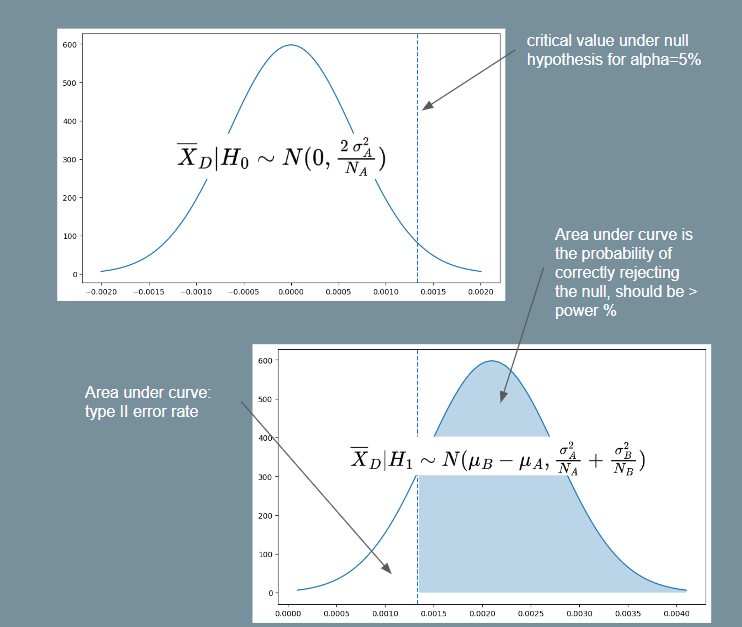 |
|---|
| Illustration for Power Analysis Derivation |
For objective 1, assuming the null hypothesis and using equation (1) above, we have . Since is a two-tailed probability and we want the critical region on the right-side, let . E.g. implies . Then:
Note that equation (2) above tells us the critical value such that we will reject the null hypothesis if the sample mean of is greater than this value. To satisfy objective 2, we must thus ensure that the probability of rejecting the null hypothesis is at least . In other words, we want . Assuming the alternate hypothesis and again using equation (1), we have . So then:
For the purpose of getting a minimum , we assume . Then using this and squaring both sides with some rearranging gives us:
Which gives us the required minimum sample size equation. If we assume , as is often assumed because we do not know the variance of the treatment, then it simplifies to the following form (as seen in Ron Kohavi's paper).
Bernoulli Events
The equation (3) above for the minimum sample size requires us to know the standard deviation under the null and alternate hypotheses. Usually, the standard deviation under the null is computed from historical data, and it is assumed that . However, if the event we are interested in may be represented as a bernoulli random variable (e.g. an impression is shown and user either clicks or does not click with some probability), the equation may be simplified.
Specifically, the variance of a bernoulli random variable with probability is . Thus, if , then , and likewise for .
So we can use and and substitute these into equation (3). We will then be able to have a minimum sample size formula by just specifying , , baseline conversion and minimum relative difference . This is the formula used by Evan Miller's sample size calculator.
Imbalanced AB Test
Another common scenario is the case where we do not split 50-50, i.e. . In this case, suppose we have , where . For example, if we have a 90-10 split, then p=9. Then we get:
Note that gives the sample size required for , and the total sample size required across both groups is .
Large Language Models
LLMs are generally used in an auto-regressive way, where the user supplies a prompt and the LLM returns a generated response. This framework makes it amenable to a wide range of tasks.
HuggingFace has a great blog post explaining how we can run LLMs on humble hardware. Typically, LLMs have billions of parameters. The following rules of thumb helps us know how much memory we need to load the LLM into memory. For a model with X billion parameters:
- Loading in
float32requires4X GBof VRAM - Loading in
bfloat16requires2X GBof VRAM - Loading in
int8requiresX GBof VRAM
Hence we see that we can load a ~7 billion parameters model with around 14GB of VRAM if loaded in bfloat16, which makes it feasible to run on GPUs like Tesla T4 with 16GB of VRAM. This can be done when loading the model with from_pretrained(..., torch_dtype=torch.bfloat16). Most models are trained in bfloat16 anyway, so it makes sense to load them at that precision.
Current popular open source LLM of that size includes mosaicml/mpt-7b, which can be easily downloaded and used using huggingface.
Quantization
It turns out that we can lower the precision of models even further than 16 bits if we use a quantization method (see e.g. Dettmers 2022, this paper is the basis for the package bitsandbytes used for quantization). The general idea is akin to encoding - we encode each number from a higher precision into a "codeword" in the lower precision (i.e. quantization). Numbers that are close to one another in the higher precision may get mapped to the same "codeword". When we want to use the encoded value, we look up the value in the higher precision that it maps to (i.e. de-quantization).
When applying this to quantizing a neural network, the steps involved are:
- Quantize all model weights to target precision (e.g.
int8) - Pass the input vector at
bfloat16 - At each layer, dequantize the weights and perform matmul in
bfloat16 - Quantize the weights again for storage
Hence while quantization lowers the memory footprint of the model, it may increase inference time. To use quantization, we need to do the following (also make sure bitsandbytes is pip installed). We can also pass load_in_4bit=True for 4bit quantization. More info on quantization usage is available at HuggingFace. An important note is that a GPU is required for quantization, at least in the bitsandbytes package.
model = AutoModelForCausalLM.from_pretrained(..., load_in_8bit=True)
Flash Attention
The self-attention mechanism (Dao 2022) is at the heart of the transformer performance but is also a major bottleneck in terms of memory and computational cost. One of the most successful optimizations for the attention mechanism is the Flash Attention paper.
Suppose we have an input sequence of embeddings where , such that . The transformer stores parameters , such that such that . The self-attention matrix is then computed to represent the pairwise interaction between tokens at position ( row) and position ( column). The row-wise softmax is taken to convert these into probabilities and finally the output is .
Typically, is much larger than the hidden dimensions , as can be 2,048 or larger. Hence the matrix is the bottleneck for memory and computation. The flash attention proposes to do this computation in a block-wise manner to reduce the memory usage. Furthermore, the algorithm also speeds up the computation compared to naive attention because the block-wise implementation minimizes the number of read-write operations between the faster SRAM and slower HBM.
More details can be found in the notebook at Dao 2022 - FlashAttention. We can utilize flash attention like so:
%pip install optimum
model.to_bettertransformer()
Note that this is only supported for models that have implemented flash attention, e.g. gpt-neox, bloom etc.
Flash Attention is now support natively within Pytorch as torch.nn.functional.scaled_dot_product_attention (see blog). The usage is like below. We need transformers>=4.36 and torch>=2.1.1 to use it.
from optimum.bettertransformer import BetterTransformer
from transformers import AutoModelForCausalLM
model = AutoModelForCausalLM.from_pretrained("gpt2-large", torch_dtype=torch.float16)
model = BetterTransformer.transform(model, keep_original_model=False)
Position Representation
Recent innovations in position encoding has led to accuracy improvements for long input sequences. The initial attention papers used absolute position embeddings. Given an input sequence of embeddings , absolute position embeddings are generated by the model. These position embeddings are added to the input sequence , thereby allowing to model to use these position cues.
It turns out that fixed positional embeddings are not ideal because they require the model to learn a fixed, unique representation of each position . This does not represent language well, because the word in position i in one sentence does not necessarily serve the same purpose as a word in the same position in another sentence. Rather, it is the relative distance between words that we want to encode in the model. Furthermore, training absolute position embeddings makes it difficult for our model to generalize to texts with longer sequences than what it was trained with.
Recent papers advocate for relative positional embeddings, with the following differences:
- Relative position encoding rather than absolute position encoding
- The encoding of relative position is done most naturally within the self-attention matrix, since that is where the relative degree of interaction between tokens at different positions is encoded
- The encoding should be such that tokens further apart have a lower value in the self-attention matrix and tokens closer together have a higher value
Rotational Position Embeddings (RoPE) (Su 2021) proposes rotating the query and key vectors by an angle proportional to the relative distance between the two positions. Specifically , where is a rotational matrix that performs the rotation.
Attention with Linear Biases (ALiBi) (Press 2022) proposes an even simpler method. It simply subtracts from row and column of the self-attention matrix, where is a fixed scalar (specific to each attention head). Intuitively, it penalizes the attention proportional to the distance between the tokens. The study shows that this method outperforms RoPE as we extrapolate to longer sequences, and is conceptually simpler.
Key-Value Cache
Most LLMs work in an auto-regressive manner, i.e. we provide an input sequence, generate the next token with the LLM, then append this token to the input sequence for the next iteration. Most LLMs are also trained with the causal language modelling objective and mask the upper triangle of the self-attention matrix, so that each query token can only interact with key token and value token if . This setup encourages us to cache results from previous time steps, since a lot of computation is repeated.
The following is based on how I imagine this to work, after reading Cameron R. Wolfe's LinkedIn post. During training, we compute the projections , where is the maximum sequence length and is the hidden dimension. The final output actually provides a -dimension representation of the model's prediction at each of the positions.
For next token generation, we can add a projection head, say , where represents the size of the vocabulary, such that can represent the activations at each of the positions for the next token. Specifically, represents the predictions of position given input tokens , represents the predictions of position given input tokens , and so on. These activations will then be fed into some cross-entropy loss such that activations at the correct token for each position gets rewarded. This allows us to do efficient training, since we simultaneously provide losses for the prediction at each of the positions to the model for backpropagation.
However, when we are doing inference generation, we only need to predict for the final position of the input sequence (suppose it is position ), i.e. we are only interested in and . Hence for starters, we only need instead of the entire matrix, since only that row comes into play. However, we still need the entire and matrices, since we want to interact with all tokens in the input sequence. This is where the KV cache comes in - we cache the existing and matrices, so that we only need to project the final token of the input sequence and at each step and append it to the existing cached and . We can then compute .
As one can imagine, this saves a lot of computation, but also increases memory costs. Kwon 2023 - PagedAttention shows that serving a 13B model on NVIDIA A100 with 40GB of memory:
- of memory is model parameters
- is the KV cache
- A small amount of memory is used ephemerally for activation
The usage of KV cache is like so:
model = AutoModelForCausalLM.from_pretrained(...)
model.generate(..., use_cache=True)
How to fine-tune an LLM
- trl RL example
- Fine tune a 20B GPT model on text generation on IMDB dataset (loaded in 8 bit)
- Since step 1 used PEFT, we need to merge the adapter weights with the base model
- Finally, use RLHF to generate positive movie reviews. They used a BERT IMDB sentiment classifer to generate rewards
- DataCamp example
- Using
SFTTrainerfrom thetrllibrary to do supervised fine-tuning
- Using
- PEFT - based on LORA - PEFT is built by hugginface to support LORA.
KV-Cache
This article walks through a simple but rigorous demonstration of KV caching in transformer autoregressive decoding.
The Attention Mechanism
In autoregressive generation, we generate tokens one at a time. Given a sequence of input embeddings , we feed the embedding matrix of size into the model to predict . Note that:
- denotes batch size
- denotes sequence length
- denotes model dimension
- denotes output vocabulary size
We will focus on the self-attention block (where the KV-cache is pertinent). For exposition, we will omit the batch size dimension for now and consider a single batch. The self attention block computes:
Where:
- (queries)
- (keys)
- (values)
The transformer produces an output of shape at the last layer. The output at the final position (call it ) is finally used to generate the logits for each token to predict like so:
Worked Example
Let's make this concrete. Suppose we have:
- 2 tokens already: (each is a 3-dimensional embedding vector)
- Projection dimension
Let's setup our input and projection matrices. Notice that each row of corresponds to one position in the sequence.
Step 1: Generate token 3 (predict given )
We compute Q, K, V for all positions:
Let's write out the full attention computation (omitting softmax and scaling for clarity):
After applying the causal mask (setting future positions to ) and softmax, we get attention weights :
Importantly, observe that the bottom row of only depends on and . is not used at all. We will see that is in fact not needed to generate the next token shortly.
Finally, the output is :
To predict , we only need the bottom row of . But this accordingly only uses the bottom row of , which only depends on . Hence, we can simplify the computation of the bottom row of as follows:
Summary: To decode for step , we need:
- Only (the query for the last position)
- All of
- All of
Now suppose we want to generate token . We will need:
Key Insight: Due to the causal mask, and did not change. Hence we can cache them and just append and to get . This is the main idea of the KV Cache.
Naive Implementation (No Cache)
Without caching, at each generation step we recompute K and V for the entire sequence:
import torch
import torch.nn as nn
import torch.nn.functional as F
def naive_attention(X, W_q, W_k, W_v):
"""
X: (batch, seq_len, d_model) - full sequence
Returns: (batch, seq_len, d_model)
"""
Q = X @ W_q # (batch, seq_len, d_k)
K = X @ W_k # (batch, seq_len, d_k)
V = X @ W_v # (batch, seq_len, d_v)
d_k = K.shape[-1]
scores = (Q @ K.transpose(-2, -1)) / (d_k ** 0.5)
# Causal mask: prevent attending to future tokens
seq_len = X.shape[1]
mask = torch.triu(torch.ones(seq_len, seq_len), diagonal=1).bool()
scores = scores.masked_fill(mask, float('-inf'))
attn = F.softmax(scores, dim=-1)
return attn @ V
def naive_generate(prompt_embeddings, W_q, W_k, W_v, W_out, num_tokens):
"""
Generate tokens without KV cache.
Each step recomputes attention over the ENTIRE sequence.
"""
X = prompt_embeddings # (1, prompt_len, d_model)
for step in range(num_tokens):
# Recompute attention for ALL positions (wasteful!)
attn_out = naive_attention(X, W_q, W_k, W_v)
# Get logits for last position only
last_hidden = attn_out[:, -1, :] # (1, d_model)
logits = last_hidden @ W_out # (1, vocab_size)
# Sample next token (simplified: just argmax)
next_token_id = logits.argmax(dim=-1)
# Embed next token and append to sequence
# (In practice, look up embedding; here we simulate)
next_embedding = torch.randn(1, 1, X.shape[-1])
X = torch.cat([X, next_embedding], dim=1)
print(f"Step {step+1}: Computed K,V for {X.shape[1]} positions")
return X
Complexity without cache: For generating new tokens with prompt length :
- Step 1: Compute K,V for positions
- Step 2: Compute K,V for positions
- ...
- Step T: Compute K,V for positions
Total K,V computations:
With KV Cache
The KV cache stores previously computed keys and values. At each step, we only compute K,V for the new token and concatenate with the cache:
def cached_attention(x_new, W_q, W_k, W_v, kv_cache):
"""
x_new: (batch, 1, d_model) - ONLY the new token
kv_cache: tuple of (K_cache, V_cache) or None
K_cache: (batch, prev_seq_len, d_k)
V_cache: (batch, prev_seq_len, d_v)
Returns: attention output, updated cache
"""
# Compute Q, K, V for the NEW token only
q_new = x_new @ W_q # (batch, 1, d_k)
k_new = x_new @ W_k # (batch, 1, d_k)
v_new = x_new @ W_v # (batch, 1, d_v)
if kv_cache is None:
K = k_new
V = v_new
else:
K_cache, V_cache = kv_cache
# Append new K,V to cache
K = torch.cat([K_cache, k_new], dim=1) # (batch, seq_len, d_k)
V = torch.cat([V_cache, v_new], dim=1) # (batch, seq_len, d_v)
# Attention: new query attends to ALL keys
d_k = K.shape[-1]
scores = (q_new @ K.transpose(-2, -1)) / (d_k ** 0.5) # (batch, 1, seq_len)
# No causal mask needed: q_new is at position seq_len,
# and we only have K,V up to seq_len (no future tokens)
attn = F.softmax(scores, dim=-1)
out = attn @ V # (batch, 1, d_v)
# Return output and updated cache
return out, (K, V)
def cached_generate(prompt_embeddings, W_q, W_k, W_v, W_out, num_tokens):
"""
Generate tokens WITH KV cache.
Two phases:
1. Prefill: Process entire prompt at once, build initial cache
2. Decode: Generate one token at a time, updating cache incrementally
"""
# === PREFILL PHASE ===
# Process entire prompt to build initial KV cache
X = prompt_embeddings # (1, prompt_len, d_model)
K_cache = X @ W_k # (1, prompt_len, d_k)
V_cache = X @ W_v # (1, prompt_len, d_v)
# Compute attention for prompt (need full Q for all positions)
Q = X @ W_q
d_k = K_cache.shape[-1]
scores = (Q @ K_cache.transpose(-2, -1)) / (d_k ** 0.5)
seq_len = X.shape[1]
mask = torch.triu(torch.ones(seq_len, seq_len), diagonal=1).bool()
scores = scores.masked_fill(mask, float('-inf'))
attn = F.softmax(scores, dim=-1)
attn_out = attn @ V_cache
last_hidden = attn_out[:, -1:, :] # Keep dim for next iteration
kv_cache = (K_cache, V_cache)
print(f"Prefill: Built cache with {K_cache.shape[1]} positions")
# === DECODE PHASE ===
for step in range(num_tokens):
# Get logits from last hidden state
logits = last_hidden.squeeze(1) @ W_out
next_token_id = logits.argmax(dim=-1)
# Embed next token (simulated)
next_embedding = torch.randn(1, 1, X.shape[-1])
# Compute attention with cache - only process NEW token!
last_hidden, kv_cache = cached_attention(
next_embedding, W_q, W_k, W_v, kv_cache
)
print(f"Step {step+1}: Computed K,V for 1 position (cache size: {kv_cache[0].shape[1]})")
return kv_cache
Complexity with cache: For generating new tokens with prompt length :
- Prefill: Compute K,V for positions (once)
- Each decode step: Compute K,V for 1 position
Total K,V computations:
Comparison
| Aspect | Without Cache | With Cache |
|---|---|---|
| K,V computations per step | ||
| Total K,V computations | ||
| Memory | ||
| Attention computation | per step |
The KV cache trades memory for computation. This is almost always worthwhile because:
- Matrix multiplications (K,V projections) are expensive
- Memory is typically available
- The speedup is dramatic for long sequences
Complete Working Example
import torch
import torch.nn.functional as F
torch.manual_seed(42)
# Dimensions
batch_size = 1
d_model = 64
d_k = d_v = 32
vocab_size = 100
prompt_len = 5
num_generate = 3
# Initialize weights
W_q = torch.randn(d_model, d_k) / (d_model ** 0.5)
W_k = torch.randn(d_model, d_k) / (d_model ** 0.5)
W_v = torch.randn(d_model, d_v) / (d_model ** 0.5)
W_out = torch.randn(d_v, vocab_size) / (d_v ** 0.5)
# Simulate prompt embeddings
prompt = torch.randn(batch_size, prompt_len, d_model)
print("=== WITHOUT KV CACHE ===")
naive_generate(prompt.clone(), W_q, W_k, W_v, W_out, num_generate)
print("\n=== WITH KV CACHE ===")
cached_generate(prompt.clone(), W_q, W_k, W_v, W_out, num_generate)
Output:
=== WITHOUT KV CACHE ===
Step 1: Computed K,V for 6 positions
Step 2: Computed K,V for 7 positions
Step 3: Computed K,V for 8 positions
=== WITH KV CACHE ===
Prefill: Built cache with 5 positions
Step 1: Computed K,V for 1 position (cache size: 6)
Step 2: Computed K,V for 1 position (cache size: 7)
Step 3: Computed K,V for 1 position (cache size: 8)
Why Only Cache K and V (Not Q)?
During autoregressive generation:
- Query (Q): We only need the query for the current position to compute attention scores. Past queries are never reused.
- Keys (K): The current query must attend to all past keys. These are reused every step.
- Values (V): Once we have attention weights, we aggregate all past values. These are reused every step.
Mathematically, for generating token at position :
Only is new. All for were computed in previous steps.
Multiple Layers: Each Layer Has Its Own Cache
Real transformers stack self-attention layers. Each layer maintains its own KV cache because:
- Each layer has different projection weights: Layer has its own and
- Each layer receives different input: The input to layer is the output of layer
Therefore, even for the same token position, the K and V values differ across layers.
def multi_layer_cached_generate(prompt_embeddings, layers, W_out, num_tokens):
"""
layers: list of dicts, each with W_q, W_k, W_v for that layer
KV cache structure: list of (K_cache, V_cache) tuples, one per layer
"""
num_layers = len(layers)
X = prompt_embeddings # (1, prompt_len, d_model)
# === PREFILL: Build KV cache for ALL layers ===
kv_caches = []
hidden = X
for layer_idx, layer in enumerate(layers):
W_q, W_k, W_v = layer['W_q'], layer['W_k'], layer['W_v']
# Compute K, V for this layer's input
K = hidden @ W_k # (1, prompt_len, d_k)
V = hidden @ W_v # (1, prompt_len, d_v)
kv_caches.append((K, V))
# Compute attention output (with causal mask)
Q = hidden @ W_q
d_k = K.shape[-1]
scores = (Q @ K.transpose(-2, -1)) / (d_k ** 0.5)
seq_len = hidden.shape[1]
mask = torch.triu(torch.ones(seq_len, seq_len), diagonal=1).bool()
scores = scores.masked_fill(mask, float('-inf'))
attn = F.softmax(scores, dim=-1)
hidden = attn @ V # Output becomes input to next layer
last_hidden = hidden[:, -1:, :]
print(f"Prefill: Built {num_layers} KV caches, each with {X.shape[1]} positions")
# === DECODE: Update each layer's cache incrementally ===
for step in range(num_tokens):
logits = last_hidden.squeeze(1) @ W_out
next_token_id = logits.argmax(dim=-1)
next_embedding = torch.randn(1, 1, X.shape[-1])
# Forward through all layers, updating each cache
hidden = next_embedding
new_caches = []
for layer_idx, layer in enumerate(layers):
W_q, W_k, W_v = layer['W_q'], layer['W_k'], layer['W_v']
K_cache, V_cache = kv_caches[layer_idx]
# Compute K, V for NEW token only at this layer
q_new = hidden @ W_q # (1, 1, d_k)
k_new = hidden @ W_k # (1, 1, d_k)
v_new = hidden @ W_v # (1, 1, d_v)
# Append to this layer's cache
K = torch.cat([K_cache, k_new], dim=1)
V = torch.cat([V_cache, v_new], dim=1)
new_caches.append((K, V))
# Attention: new query attends to all cached K, V
d_k = K.shape[-1]
scores = (q_new @ K.transpose(-2, -1)) / (d_k ** 0.5)
attn = F.softmax(scores, dim=-1)
hidden = attn @ V # (1, 1, d_v) - input to next layer
kv_caches = new_caches
last_hidden = hidden
cache_size = kv_caches[0][0].shape[1]
print(f"Step {step+1}: Updated {num_layers} caches (each now size {cache_size})")
return kv_caches
Memory for KV cache with layers:
The factor of 2 is for K and V. For large models (many layers, large ), this becomes the dominant memory cost during inference.
Example: Llama 2 70B has:
- layers
- per head, 64 heads → 8192 total
- For a 4096-token sequence in fp16:
This is why KV cache compression techniques (quantization, eviction, etc.) are active research areas.
References
Automatic Prompt Optimization
Automatic prompt optimization is a research area of recent interest. This trend arises from the following observations:
- Adjusting textual prompts can very significantly change LLM's ability to accurately complete tasks
- The correlation between prompt and performance is not always the most obvious or intuitive to humans
- The best prompt varies depending on the LLM model (or even different iterations of the same model)
LLMs are increasingly used to solve diverse problems by varying the instructions. This is often a simpler solution than maintaining many models that do various specific tasks. For example, in the recsys world, companies like LinkedIn and Netflix are moving toward foundational LLM models that can replace a collection of traditional recommender models. By adjusting the instructions to the foundation model, it can achieve comparable or even better performance to these task-specific models due to favourable scaling laws with the size of the model.
However, manually tuning the instruction for each task is brittle and model performance can easily change as the underlying foundation model is continually trained and improved, or swapped out. Also, we may often want to adapt a foundational model to a new task without performing further fine-tuning or training adapter weights. Hence, automatic prompt optimization becomes an important tool to maintain model performance in an operational setting.
This note focuses on gradient-free methods to optimize black-box LLMs, as they are often simpler and are applicable to LLM usage via API, which is still the most common LLM usage method outside of big tech companies. I also follow Wolfe 2024 heavily but simplify quite a bit for readability.
Main Idea
The main idea of automatic prompt optimization is to simply treat the task of prompt optimization as a standard machine learning problem. That is, we construct a training dataset and optimize our prompt to improve performance on it, and validate the effectiveness of the prompt on a held out validation set. The only difference is that we have to be creative in how we optimize the prompt, since we cannot use gradient descent to do so.
Specifically, the general setup that we consider is such:
- We have a dataset of inputs and labels that can be split into train and validation sets
- Labels are optional if we are using another LLM as judge
- For each training example, we can produce textual output from an LLM call:
- We have some evaluation function that returns a score for this example instance:
- The evaluation function obviously depends on the specific task
- E.g. for simple tasks, the evaluation function can simply be the accuracy of
- The evaluation function can also be another LLM for ambiguous tasks
- We can thus compute the mean score across a set of training instances to evaluate the effectiveness of a given prompt
- At each iteration, we try one or more new prompt(s) and evaluate their performance, then have some way of generating new prompts to try again
- At the end, the best prompt is selected
Methods
Here we dive into the different methods. Some are quite ingenious in how they use LLMs to elicit the best instructions. Note that we omit papers that perform prompt optimization through some gradient-based optimization (e.g. using reinforcement learning), as these cannot be used with LLMs accessed through API.
Instruction Induction
Honovich 2022 is an early paper that suggests taking a random subset of training (input, label) pairs, showing them to an LLM, and asking the LLM to guess the instruction that produces the label from the inputs.
For example, the LLM prompt may look something like:
Here are the input-output pairs:
Input: As soon as you can.
Output: At your earliest convenience.
...
The instruction was <PLS FILL IN>
The LLM may then guess something like The instruction was translate the inputs into more formal language. We can then use this instruction as the new optimized prompt.
Note that this method is a one step process, i.e. it does not iterate for further improvements. But I suppose we can sample multiple random subsets of training instances and generate prompts for each before picking the best prompt.
Bibliography
- Honovich 2022: Instruction Induction
- Yang 2023: Large Language Models as Optimizers (OPRO)
- Wolfe 2024: Automatic Prompt Optimization
Fine-tuning
LLMs are typically trained with next-token prediction task on large amounts of text in an unsupervised manner. Some of the behaviour in these texts are not desirable to imitate. For example, while Github is full of code repositories with common programming mistakes, we do not want the LLM to replicate such behaviour. Hence, a process of alignment is necessary to encourage the model to produce desired responses.
There are typically two stages to this fine-tuning: Supervised Fine-Tuning and Reinforcement Learning from Human Feedback.
Supervised Fine-Tuning (SFT). In this stage, pairs of (prompt, desired response) are provided to the LLM. The desired responses are often called "demonstrations" by human annotators. Some form of cross-entropy loss is then used to update the LLM to encourage it to generate the desired response. This is a straightforward approach that is similar to the next-token prediction task (except we are predicting the desired response given the prompt). In the InstructGPT paper, the authors show that an SFT-aligned 1.3B model (using ~13k training data) generates human-preferred outputs compared to a 175B GPT model, showing the importance of SFT.
The problem with SFT is that it trains the model to provide a very specific response to a particular prompt, which makes it hard for the model to generalize. It also fails to express the natural ambiguity of responses for an open-ended prompt (e.g. write a poem about AI). Hence, unless we can collect quality responses for a very wide variety of prompts, SFT is limited in its ability to generalize.
Reinforcement Learning from Human Feedback (RLHF). This is where RLHF comes in: given triplets of (prompt, preferred response, not preferred response), we train the model to generate the preferred response in a more generalizable way.
More recently, a method called Direct Preference Optimization is used to solve this problem without needing to do reinforcement learning. More on that here.
Useful Models
There are too many models on Huggingface, so I try to keep track of useful ones here. Generally the open_llm_leaderboard is a good place to start.
| Model Name | # Params (Billions) | openllm score | Comments |
|---|---|---|---|
| SOLAR-10.7B-Instruct-v1.0 | 10.7B | 74.2 | This model was trained using Supervised Finetuning (SFT) and Direct Preference Optimization (DPO) for single-turn chat. Seems to be derived from Llama. Verified that the outputs are sensible. |
Testing SOLAR-10.7B
Here are some results from testing out SOLAR-10.7B-Instruct-v1.0 on Google Colab, with a T4 GPU. First we install packages and load the model. Note that we are quantizing it to 4bits to save memory, and specifying the compute type of torch.float16 as that is the tensor type that this model was trained in. Using torch.float32 (which is the default) will incur unnecessary conversion cost and slow down inference.
%pip install transformers~=4.36 torch~=2.1.1 bitsandbytes accelerate optimum
from transformers import AutoModelForCausalLM, AutoTokenizer, BitsAndBytesConfig
import torch
quantization_config = BitsAndBytesConfig(
load_in_4bit=True,
bnb_4bit_compute_dtype=torch.float16
)
MODEL_NAME = "Upstage/SOLAR-10.7B-Instruct-v1.0"
tokenizer = AutoTokenizer.from_pretrained(MODEL_NAME)
model = AutoModelForCausalLM.from_pretrained(
MODEL_NAME,
device_map="auto",
quantization_config=quantization_config,
)
We define a generate function.
def generate(prompt: str, max_length: int = 2048):
conversation = [{'role': 'user', 'content': prompt}]
prompt = tokenizer.apply_chat_template(conversation, tokenize=False, add_generation_prompt=True)
inputs = tokenizer(prompt, return_tensors="pt").to(model.device)
outputs = model.generate(**inputs, use_cache=True, max_length=max_length)
output_text = tokenizer.decode(outputs[0])
return output_text
And now we can test it out on a few prompts.
Prompt: Can you explain web3 to a 5 year old? Response: Web3 is like a special world on the internet that lets people share and use things in a new and more open way. Imagine a playground where everyone can add their own swings, slides, and sandboxes without needing permission from a big boss. This makes it easier for people to work together and create new fun things online. (Inference time: 8s)
Prompt: Can a firefighter transit into the finance industry? Response: While it may not be a typical career transition, it is possible for a firefighter to transition into the finance industry. To make a successful move, the firefighter would need to acquire the necessary skills and qualifications relevant to the finance sector. This could involve pursuing additional education or training in finance, accounting, or business administration. Networking, gaining relevant work experience, and showcasing transferable skills from the firefighting profession can also help in making the transition.\n\nSome transferable skills from firefighting to finance could include strong problem-solving abilities, teamwork, decision-making under pressure, and the ability to manage risk. However, it's essential to note that the finance industry has its unique requirements, and the firefighter would need to demonstrate a strong commitment to learning and adapting to the new environment. (Inference time: 19s)
Seems to be pretty decent performance at a somewhat reasonable inference time out of the box.
Gemma Models
References:
Google released open source small models under the Gemma label. It comes in two sizes: 2B and 7B parameters, each with base (pretrained) and instruction-tuned versions. All have a context length of 8k tokens. Gemma integration is supported with transformers==4.38. Note that user consent is needed to access Gemma models, so one needs to create a HuggingFace account and create an access token.
Sample Code
# Use model_name="google/gemma-7b-it"
def load(model_name: str):
tokenizer = AutoTokenizer.from_pretrained(model_name, token=TOKEN)
model = AutoModelForCausalLM.from_pretrained(
model_name,
quantization_config=BitsAndBytesConfig(
load_in_4bit=True,
bnb_4bit_compute_dtype=torch.bfloat16,
bnb_4bit_use_double_quant=True, # nested quantization
bnb_4bit_quant_type="nf4", # normalized quantization
),
token=TOKEN,
)
return model, tokenizer
Inference Speed
Tested out the inference speed of the model using the following prompt: Can you recommend good alternative occupations for a occupation_name? Please be concise.
An example is as follows, for an occupation counsellor:
Sure, here are some alternative occupations for a counsellor:
* **Social worker:** Similar to counselling, social workers help individuals and families facing various challenges.
* **Community organizer:** Organizes and leads community initiatives to address social issues.
* **Teacher:** Can be a good fit for those who enjoy working with children and adolescents.
* **Human resource manager:** HR managers handle employee relations and conflicts.
* **Public relations specialist:** Helps organizations communicate effectively with the public.
The inference speed is about 8-10 seconds with 4-bit quantization.
Gemma-2b
Testing out google/gemma-2b-it shows that it has poorer performance but faster inference speed at 2 billion parameters. Here is an example of the results for the same prompt.
* **Life coach**
* **Coach in education**
* **Career coach**
* **Executive coach**
* **Leadership coach**
* **Management consultant**
* **Business development consultant**
* **Financial advisor**
* **Investment banker**
The inference speed is as follows:
- Single:
3s - Batch of
4:14s - Batch of
8:16s - Batch of
16:20s - Batch of
32: OOM on T4 GPU
Phi-2
Mobius Labs fine-tuned the phi-2 model from Microsoft which seems promising, and released it under mobiuslabsgmbh/aanaphi2-v0.1. The output seems better than gemma-2b-it.
1. Social worker
2. Mental health therapist
3. School counselor
4. Employee assistance program (EAP) specialist
5. Rehabilitation counselor
6. Family therapist
7. Substance abuse counselor
8. Career counselor
9. Trauma-focused therapist
10. Child and adolescent therapist
These occupations involve working with individuals, families, and communities to promote mental health and well-being, and may provide similar skills and experiences to those of a counsellor.
Flash attention, torch.compile, quantization.
Encoder vs Decoder
There are broadly two categories of LLMs: Encoder-Decoder architecture (typified by BERT) and Decoder only architecture (typified by GPT-2 series). There are some innate differences between the two that affect the type of application each is well suited for.
Encoder-Decoder Architecture
The Encoder-Decoder architecture was proposed in the original Attention is All You Need paper by Vaswani et al. As the name suggests, there is a separate encoder and decoder module. The design choice of two distinct modules is easier to understand when we consider that the original paper was designed for the machine translation task, such that the inputs may be in English and the outputs may be in French.
On the encoder-side, the encoder module sees the full input sequence and encodes it into an numeric encoding representation matrix of size (seq_len, embed_dim). There is no input masking required because we assume we see the full English text before we begin translation. This encoding representation is passed to the decoder module as context.
On the decoder-side, we cannot allow the decoder module to see the full output sequence during training, since that would cause data leakage and the model to collapse. Note that the decoder simultaneously (in one forward pass) predicts a token for each position in the output sequence during training. Hence to avoid data leakage, causal masking is applied such that for each position being predicted, the decoder module is only allowed to "see" tokens in previous positions.
Note that this can be implemented simply by masking the attention matrix in each self-attention block in a triangular manner. The feedforward layers only map information from position i to position i, so there is no need to adjust that.
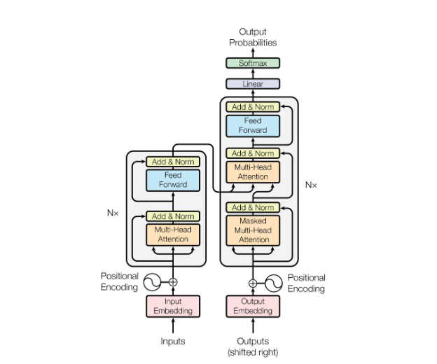 |
|---|
| BERT Encoder Decoder Architecture (From Attention is All You Need) |
The decoder module itself creates a representation of the output sequence (with causal masking) of size (seq_len, embed_dim). Now for the tricky part of merging the encoder and decoder representations. Naively, we can simply concatenate the two to form a representation of (seq_len x 2, embed_dim), and add further self-attention blocks (with appropriate causal masking). However, this would increase the number of parameters of the model.
The paper instead chose to take the Q matrix from the decoder and the K, V matrices from the encoder. Since the attention mechanism is , this allows every token on the decoder representation to attend to every token on the encoder representation. The result is a weighted combination of the V vectors taken from the encoder representation which is eventually used to generate the tokens for each decoder position.
Here we can already observe some inductive biases baked into the encoder-decoder architecture. These comments are inspired by / taken from Hyung Won Chung's lecture:
- There is a clear distinction between the tokens on the encoder-side and the decoder-side, such that tokens on either side cannot directly attend to each other until the final block when the mixing happens. This may be suitable for the translation task but not for generic chat completion, where it is quite arbitary which point in the conversation we determine as the encoding and which point we determine as the decoding.
- The
Vmatrix is taken entirely from the encoder-side, which may again limit the expressiveness of the model (what if there are important tokens on the decoder-side that would be useful to taken theVvalues from?). One may argue that in translation, the tokens on the encoder-side capture the full meaning of the sentence to be translated, so it is comprehensive. But the same is not true of generic chat completions. - The separation of an encoder and decoder module suggests that there is significant difference between the tokens on the encoder-side and decoder-side. Again, this inductive bias
Contextualized Recommendations
Contextualized recommendations is an emerging use case from LLMs. The idea is that we use a traditional search and recommender system to generate recommendations, and use an LLM to craft an explanation for why each recommendation is relevant to the user in a very personalized way. Multiple companies have reported that this has driven engagement and clicks up significantly.
Spotify
Contextualized recommendations through personalized narratives using LLMs
Traditionally, spotify users use just the cover art to decide whether to engage with a new music recommendation. Spotify wants to include a short one-liner to explain why a particular item might resonate with users. For example, Dead Rabbitts latest single is a metalcore adrenaline rush! or Relive U2's iconic 1993 Dublin concert with ZOO TV Live EP.
Spotify highlights some challenges they faced:
- Ensuring a consistent generation style and tone
- Avoiding harmful or inappropriate outputs
- Mitigating hallucinations and inaccuracies
- Understanding user preferences to deliver tailored meaningful explanations
Initial tests with zero-shot / few-shot Llama did not work too well. They adopted a human-in-the-loop approach:
- Expert editors provide "golden examples" for instruction fine-tuning
- Provide ongoing feedback to address errors in LLM output
- Artist attribution errors
- Tone inconsistencies
- Factual inaccuracies
The AB tests showed that explanations containing meaningful details about the artist or music led to significantly higher user engagement.
For LLM fine-tuning, they found that Llama 3.1 8B worked well and could be trained with multiple adapters for 10 different tasks. Throughout the training process, they used MMLU benchmark as a guardrail to ensure that the model's overall ability remained intact. Spotify uses vLLM for inference.
LinkedIn provides AI features for premium users. When users click on a job, they can ask questions like "Am I a good fit for the job?". The LLM will respond with a short bullet-pointed explanation on:
- Whether the user is a good fit
- Details from the user's profile that make them a good fit
- Areas that the users are missing
MinGPT
This is a walkthrough of KArpathy's MinGPT implementation
bpe.py
This file contains code to implement a Byte Pair Encoding encoder. It does not contain code for training, just loads openai's GPT-2 bpe encoding for inference.
Most text is represented in UTF-8 encoding, which is just a sequence of bytes (values 0 to 255). For example, 0xf0 corresponds to 33 in decimal which corresponds to the character !. This means that all text can be treated as a sequence of byte values.
As a fallback, we first need token representations for individual byte values (in case we encounter out of vocab tokens with unknown byte sequences).
First, two files are downloaded in get_encoder, from https://openaipublic.blob.core.windows.net/gpt-2/models/124M/:
encoder.jsonis a dict of len50257mapping from a token to its index. This represents the entirety of the vocabulary- The first
256tokens represents the256byte values. Each token is some arbitrarily chosen character (just need to make sure it is printable) - These tokens are a fallback to ensure that we can encode any text sequence. For example, if we encounter a new emoji with unknown byte sequence, at the very least we can encode each byte separately.
- The next
50ktokens map from a byte sequence of length2and above to an index, these are the BPE mined sequences of merged bytes - The last token is
<span class="hl-subtle">endoftext</span>which is a special token
- The first
vocab.bpeis a\nseparated list of byte sequences that should be merged (50kof them)- In contrast to the above, these sequences are not merged yet (e.g. a line is
R ocket) - We store these as a
list[tuple]inbpe_merges
- In contrast to the above, these sequences are not merged yet (e.g. a line is
These two data are passed into the Encoder main class.
Statistics
Conformal Predictions
Exchangeability
In this section we discuss the difference between independence and exchangeability.
Definition. Independence.
Two events and from a sample space are said to be independent if .
If , it is equivalent to say , since:
Definition. Exchangeability
Two events and are said to be exchangeable if , which means there is indifference with respect to the order of events.
More generally, exchangeability of a sequence of events means that the joint distribution is unchanged when we permute the order of events:
The simplest way to understand is to use the example of drawing balls from an urn without replacement (example taken from Cordani 2006). Suppose we have an urn with 10 red balls and 5 white balls. Then the following tree shows the draw probabilities at each step:
graph TD;
A((Start)) --> R1("R1 (10/15)");
A --> W1("W1 (5/15)");
R1 --> R2("R2 (9/14)");
R1 --> W2("W2 (5/14)");
W1 --> R2_2("R2 (10/14)");
W1 --> W2_2("W2 (4/14)");
R2 --> R3("R3 (8/13)");
R2 --> W3("W3 (5/13)");
W2 --> R3_2("R3 (9/13)");
W2 --> W3_2("W3 (4/13)");
R2_2 --> R3_3("R3 (9/13)");
R2_2 --> W3_3("W3 (4/13)");
W2_2 --> R3_4("R3 (10/13)");
W2_2 --> W3_4("W3 (3/13)");
Suppose we
References
Miscellaneous Notes
A collection of miscellaneous, useful notes.
f-strings
To surround a text with a symbol (say =) to a fixed length:
>>> text = "Title"
>>> print(f"{text:=^20}")
=======Title========
Vim
Command to interactively change each 'foo' to 'bar'. :%s triggers the substitute global command, followed by the search and replace phrases respectively. Finally g means replace all occurrences and c means with confirmation. Note that :s will only do the same for one line.
:%s/foo/bar/gc
Find Files
To find files anywhere on the system with the filename python using bash, use:
find . -name python
We can add * before and/or after the filename to allow other characters before or after our keyword:
find . -name *python*
To search not just in the filename but also in the full path (e.g. we only want to search in Desktop), we can do:
find . -wholename "*Desktop*python*"
Note that if we want to locate executable binaries, another useful command is whereis:
whereis cat
---
cat: /usr/bin/cat /usr/share/man/man1/cat.1.gz
Numpy Indexing
Suppose we have a 2D array X and would like to take a slice of certain rows and columns. We might try, for e.g., to take the first two rows of X and the 3rd/4th column of X, i.e. we expect to get a 2 by 2 matrix.
import numpy as np
X = np.random.randn(5, 5)
X[[0, 1], [2, 3]]
Unfortunately, this will return an array of items array(X[0, 2], X[1, 3]), which is not what we want. Instead, a slightly inefficient but clear way is to slice each axis separately. It is not optimal because the first slice creates a temporary array view before the second slice is applied.
X[[0, 1], :][:, [2, 3]]
Finally, the recommended way seems to be to use np.ix_. Doing np.ix_([0, 1], [2, 3]) creates a tuple of two elements.
idx = np.ix_([0, 1], [2, 3])
idx
>> (array([[0],
[1]]),
>> array([[2, 3]]))
Indexing the original array with this output X[idx] will then give us what we want.
asyncio
asyncio is a single-threaded framework that does not use multi-threading or multi-processing to speed up tasks. Instead, a coordinator (or event loop) passes control from a time-consuming blocking function (e.g. time.sleep or an I/O operation) to other functions to run. This passing of control occurs with the await keyword. When the blocking function is completed, it notifies the coordinator and control returns to where the blocking function left off.
asyncio does not speed up CPU-bound tasks, due to its single-threaded design. It only works when the function being awaited is an I/O operation that is supported by asyncio. This includes stuff like:
- HTTP (supported through
aiohttp) - DB calls (e.g.
aioredis)
asyncio is preferred for such tasks (e.g. making multiple I/O calls and doing something when they all return) over multi-processing because of its single-thread design, making it easier to debug.
relatedness
In the context of information retrieval, Trey Grainger in AI-Powered Search suggests a relatedness measure to connect arbitrary entities together. Suppose we have a collection of jobs and each job is tagged with a set of skills. Suppose we wish to retrieve relevant skills to an arbitrary free text query .
The relatedness idea is to define a foreground of documents, e.g. based on a retrieval of documents using query which are related to the query, and to compare the attributes of the foreground against the background, i.e. all documents.
Mathematically, we can think of the foreground documents as a sample, and the background documents as the population. The strength of the relationship between each skill to the query may then be defined as the z-statistic of the one-sample z-test of proportions of the occurrence of skill in the foreground sample compared against the background population. A significantly greater occurrence in the sample compared to the population suggests a strong relationship between and , and vice versa. Specifically:
Where:
- is the sample proportion.
- is the number of documents in the foreground corresponding to query and contains skill .
- is the total number of documents in the foreground corresponding to query . It is also the number of samples .
- is the probability of skill t appearing across all documents.
By performing a retrieval and ranking skills based on the z-statistic, we can compute a relationship between any arbitrary query and attribute of the documents (on the fly, if necessary). This functionality is implemented in solr.
Package Versioning
SemVer is the versioning standard for Python packages. For a package version of e.g. 1.2.3:
- The first number
1is the major version. We update it when we make major API changes. A major of0indicates that the package is under initial development and anything may change. - The second number
2is the minor version. We update it when we add functionality in a backward compatible manner. - The third number
3is the patch version. We update it when we patch bugs in a backward compatible manner.
Poetry is a useful tool to manage package dependencies in a Python library. In the pyproject.toml file, we specify package dependencies in the following manner:
[tool.poetry.dependencies]
python = ">=3.8,<3.11"
requests = "^2.26.0"
pytz = "~2022.1"
The caret requirement (e.g. requests = "^2.26.0") means that SemVer compatible changes are allowed, i.e. an update is allowed if the version number does not modify the left-most non-zero digit. E.g.:
^1.2.3means that1.3.0is allowed but not2.0.0^0.2.4means that0.2.5is allowed but not0.3.0
The tilde requirement is somewhat stricter. It specifies a minimal version but allows room to upgrade depending on how many digits are supplied. If major.minor.patch or major.minor is supplied, only patch-level changes are allowed. If major is supplied, minor and patch level changes are allowed.
~1.2.3means that1.2.7is allowed but not1.3.0~1.2means that1.2.7is allowed but not1.3.0~1means that1.3.0is allowed but not2.0.0
The poetry versioning specification depends on developer updating the library versions in a disciplined way. It allows us to provide some flexibility in package versioning while avoiding updating a dependent package to a version that breaks our code. Having more flexibility in specifying package dependencies reduces the risk of dependencies version conflicting.
Parallelism in Python
References: realpython, superfastpython
The Python Global Interpreter Lock (GIL) is a lock that allows only one thread to run at a time. The reason for this design feature in Python is because the Python interpreter is not thread-safe, meaning that if the GIL did not exist, the Python interpreter could introduce race conditions and other fatal errors due to multiple threads modifying memory at the same time. The GIL also allowed other non-thread-safe C programs to be easily integrated into the Python ecosystem, which contributed to Python's success as a language.
The GIL also improves performance for single-threaded programs, as it only requires a single lock to be managed (not sure how this works). There have been attempts to remove the GIL from Python but none have been successful because they would degrade single-threaded performance.
For many C extensions (e.g. numpy), multi-threading is still possible because these extensions are allowed to manually release the GIL (as long as they restore things back to normal when the functions return). This allows us to still use multi-threading for CPU-intensive functions with the GIL around. Similarly for Rust, we can release the GIL to achieve parallelism.
Alternatively, we can use multiprocessing to create multiple processes (instead of threads). Each process contains its own Python interpreter (and GIL) and hence can run truly in parallel. The downside is that the overhead of creating and managing processes is much more than that for threads, meaning that the benefits of multiprocessing are much dampened compared to multi-threading.
Memory Profiling
It is often useful to profile the memory usage of our script. In python, we can use memory_profiler to check the memory usage of our program line by line.
from memory_profiler import profile
import sys
@profile(stream=sys.stdout)
def f():
a = [1] * (10**6)
b = [2] * (2 * 10**7)
del b
if __name__ == "__main__":
f()
This will print the following useful information to stdout. Note that even before we did anything, there is background memory usage of 17MiB.
Filename: memory_profiling.py
Line # Mem usage Increment Occurrences Line Contents
=============================================================
5 17.1 MiB 17.1 MiB 1 @profile(stream=sys.stdout)
6 def f():
7 24.5 MiB 7.5 MiB 1 a = [1] * (10**6)
8 177.2 MiB 152.6 MiB 1 b = [2] * (2 * 10**7)
9 24.8 MiB -152.4 MiB 1 del b
We might also want to track memory usage of a function over time. We can use memory_usage instead for that.
import time
from memory_profiler import memory_usage
def g(a, n: int = 100):
time.sleep(1)
b = [a] * n
time.sleep(1)
del b
time.sleep(1)
if __name__ == "__main__":
usage = memory_usage((g, (1,), {"n": int(1e7)}), interval=0.5)
print(usage)
This will give us an array like so, showing the spike in memory in the middle of g.
[17.375, 17.5234375, 17.5234375, 19.34765625, 93.59765625, 93.59765625, 17.53125, 17.53125, 17.53125]
CUDA
PyTorch may sometimes throw errors if the installed torch version does not match the installed CUDA version. To address this, we need to first check the CUDA version using the nvcc command:
/usr/local/cuda/bin/nvcc --version
---
nvcc: NVIDIA (R) Cuda compiler driver
Copyright (c) 2005-2022 NVIDIA Corporation
Built on Wed_Jun__8_16:49:14_PDT_2022
Cuda compilation tools, release 11.7, V11.7.99
Build cuda_11.7.r11.7/compiler.31442593_0
Then install the correct version of torch:
pip install -U torch torchvision torchaudio --index-url https://download.pytorch.org/whl/cu118
List Comprehension
When doing nested list comprehensions in python, the later loop becomes nested as the inner loop. So this:
l = [i * j for i in range(4) for j in range(5)]
Is equivalent to:
l = []
for i in range(4):
for j in range(5):
l.append(i*j)
This also explains why flattening a list of lists is of the following form:
list_of_lists = [[0, 1, 2], [3, 4, 5], [6, 7, 8]]
flattened = [item for sublist in list_of_lists for item in sublist]
When we translate it into a nested for loop, we can see that the inner loop should indeed be placed at the end:
flattened = []
for sublist in list_of_lists:
for item in sublist:
flattened.append(item)
Configure VsCode Snippets
When typing stuff in VsCode, we sometimes write the same boilerplate and want to have a shortcut to type it for us. For example, when writing latex, we often have to create an align environment like so:
$$
\begin{align*}
Equations go here..
\end{align*}
$$
VsCode has a snippets function to help us with that.
- Press
Ctrl + Shift + Pand typeConfigure User Snippets - Create a local or global snippets file and name it (e.g.
charles.code-snippets) - Add the snippet definition like the below
{
"LaTeX Align Environment": {
"prefix": "align",
"body": [
"$$",
"\\begin{align*}",
"\t$1",
"\\end{align*}",
"$$$0"
],
"description": "Inserts a LaTeX align* environment."
}
}
Note that the prefix is the keyword to trigger the template. To use the template, we simply enter insert mode in vim as per normal (e.g. using a or i or o), then type align. At this point, we would see the text as per normal. We can then press ctrl+space to show the snippets auto-completion, if there are any. Finally, we just press enter to get the template generated. The cursor will now come to rest at position $1 as indicated in the snippet.
Github in Colab
We may want to run .ipynb notebooks within a github project in colab. There are two steps to this.
First, to get the .ipynb itself into colab, we can either use the UI to manually upload the notebook, or if we are loading from Github, we can simply start with the url to the notebook https://github.com/charleslow/REPOSITORY/blob/master/NOTEBOOK.ipynb and change github to githubtocolab. This will automatically open up the notebook in colab.
However, this only gives us the standalone notebook, and we will not have access to the project directory and packages. Hence, in the notebook, we need to:
!git clone <Insert REPOSITORY name>.git%cd folder name
This will allow us to import packages and run the notebook as per normal.
Quartz Cron
We often use quartz cron expressions to schedule jobs. A cron expression is simply 6 or 7 values in a space-separated string, such as:
"0 0 0 1 * ?"
Which means run on the:
0th secondof the0th minuteof the0th hourof the1st day the monthofevery month- and doesn't matter which
day of the week
The specifics of each field are in the table below, from the cron trigger tutorial:
| Field Name | Mandatory | Allowed Values | Allowed Special Characters |
|---|---|---|---|
| Seconds | YES | 0-59 | , - * / |
| Minutes | YES | 0-59 | , - * / |
| Hours | YES | 0-23 | , - * / |
| Day of month | YES | 1-31 | , - * ? / L W |
| Month | YES | 1-12 or JAN-DEC | , - * / |
| Day of week | YES | 1-7 or SUN-SAT | , - * ? / L # |
| Year | NO | empty, 1970-2099 | , - * / |
On the special characters:
*is commonly used, meaning "select all the values"?is only used for Day of month or Day of week. Basically if we set one, we must set the other to?to avoid a conflict-is used to specify a range. E.g.10-12in the hour field means run on the10th,11thand12thhour,is used to specify a few values, e.g.10,12n the hour field means run on the10thand12thhour/is used to specify increments. e.g.0/15in the minutes field means run on minutes0, 15, 30, 45#is a special case for Day of the Week. Basically,MON#1means the 1st occurrence of a Monday of the given month
That's about it! Or we can just use an LLM to generate the expression we need.
Wayland in Devcontainer
Sometimes we may encounter this error when trying to use vscode to setup a devcontainer:
Error response from daemon: invalid mount config for type "bind": bind source path does not exist: /run/user/1000/wayland-0
This happens because VS Code is trying to share the graphics connection with the container, which is not needed in most cases. Here is how to disable it:
- Open VS Code Settings
(Ctrl + ,) - Search for "Mount Wayland Socket"
- Uncheck the box for Dev > Containers: Mount Wayland Socket
- Rebuild your container (Ctrl + Shift + P -> "Rebuild Container").
Bradley-Terry Model
Based on wikipedia. The Bradley-Terry model (1952) is a probability model that allows us to infer scores for individual objects based on a dataset of pairwise comparisons between them. Specifically, it estimates the probability that (i.e. is preferred to ) as:
Where is a positive real-valued score assigned to object (not necessarily a probability). Typically, is parametrized as an exponential score , and the goal is to learn the parameters from pairwise comparisons. This results in:
Parameter Estimation
Parameter estimation is typically done using maximum likelihood. Starting with a set of pairwise comparisons between individual objects, let be the number of times object beats object . Then the likelihood of a given set of parameters ( denotes number of objects) is as follows:
This likelihood function can then be minimized by differentiating wrt and solved by setting to zero.
BT Model as a Sigmoid Function
We can also express the likelihood as a function of the difference in scores . Recall that the sigmoid function is . Then:
The derivation for the second line above is found at /Identities/sigmoid. This re-parametrization shows that the BT-model is really modelling the preference as a difference in scores and then running that through the sigmoid function to convert it into a probability. This means that we are basically running a pairwise logistic regression.
Setting up WSL
We may need to uninstall and re-install WSL (Windows Subsystem for Linux) from time to time. Here is the step-by-step.
- Tear down and delete all files.
wsl --unregister Ubuntu-22.04 - Re-install wsl.
wsl --install Ubuntu-22.04 - Set up keychain to auto-find ssh-agent (from Windows) and add keys
- Copy
.sshfolder from Windows to wsl~/.ssh - Add to
~/.bashrcthe following:eval $(keychain --eval --agents ssh id_rsa)
- Copy
- Install Docker
- Add users to docker to allow vscode access
- https://docs.docker.com/engine/install/linux-postinstall/
- Essentials (get C linker)
sudo apt install build-essential
- Install rust
- https://www.rust-lang.org/tools/install
- Install mdbook
cargo install mdbook mdbook-katex
ssh-agent forwarding
One challenge in WSL is to forward the ssh-agent from WSL into the devcontainer. Make sure to include the following in devcontainer.json for this to happen.
{
"customizations": {
"vscode": {
"settings": {
"remote.containers.sshForwardAgent": true
}
}
}
}
Configure Blackout
It's useful to have a screen blackout command to keep jobs running but not show our screen when leaving the desk.
Click New and create a shortcut, paste the following command:
powershell.exe -Command "(Add-Type '[DllImport(\"user32.dll\")]public static extern int SendMessage(int hWnd, int hMsg, int wParam, int lParam);' -Name a -Pas)::SendMessage(-1,0x0112,0xF170,2)"
Set the shortcut name (e.g. blackout). Finally, add a keyboard shortcut to it (e.g. Ctrl + Alt + B).
To Read
- https://netflixtechblog.com/improve-your-next-experiment-by-learning-better-proxy-metrics-from-past-experiments-64c786c2a3ac
- https://netflixtechblog.com/sequential-a-b-testing-keeps-the-world-streaming-netflix-part-1-continuous-data-cba6c7ed49df
- https://arxiv.org/abs/2407.02464
- https://arxiv.org/abs/2305.12102
- https://arxiv.org/abs/1709.03933
- https://arxiv.org/abs/2101.08769
- https://arxiv.org/abs/1205.2618 # BPR
- https://arxiv.org/abs/2312.08520 # InfoNCE+
- https://arxiv.org/abs/2308.06091 # MAWU
- https://arxiv.org/abs/2109.12613 # CCL
- https://arxiv.org/abs/2201.02327 # SSM
- https://arxiv.org/abs/2206.12811 # DirectAU
- KG-BERT
- XR-Transformer
- SetFit
- Lora vs Fine tuning
- Better Generalization with semantic IDs
- Mutual Information Neural Estimation
- Contrastive Learning with Hard Negatives
- Decoupled Contrastive Learning
- Improving Graph Collaborative Filtering with Neighborhood-enriched Contrastive Learning
- Semi-Supervised Classification with Graph Convolutional Networks
- Ranking Distillation
- PinnerFormer
- BERT4Rec
- Retrieval as Attention
- Generate Rather than Retrieve
- PLM in Baidu Search
- Emebdding Based Retrieval in Facebook Search
- Self Attentive Sequential Recommendation
- Is BERT4Rec really better than SASRec?
- Transformers4Rec
- Pretrained Transformers for Text Ranking: BERT and Beyond
- Turning Dross Into Gold Loss: is BERT4Rec really better than SASRec?
- Modularized Transfomer-based Ranking Framework
- Pre-trained Language Model for Web-scale Retrieval in Baidu Search
- Related Pins at Pinterest: The Evolution of a Real-World Recommender System
- Improving Pinterest Search Relevance Using Large Language Models
- Pixie: A System for Recommending 3+ Billion Items to 200+ Million Users in Real-Time
- Towards Personalized and Semantic Retrieval: An End-to-End Solution for E-commerce Search via Embedding Learning
- Ranking Relevance in Yahoo Search
- Fine-Tuning LLaMA for Multi-Stage Text Retrieval
- Revisiting Deep Learning Models for Tabular Data
- OmniSearchSage: Multi-Task Multi-Entity Embeddings for Pinterest Search
- Search-based User Interest Modeling with Lifelong Sequential Behavior Data for Click-Through Rate Prediction
- Behavior Sequence Transformer for E-commerce Recommendation in Alibaba
- Graph Convolutional Neural Networks for Web-Scale Recommender Systems
- PinnerSage: Multi-Modal User Embedding Framework for Recommendations at Pinterest
- ItemSage: Learning Product Embeddings for Shopping Recommendations at Pinterest
- RankT5: Fine-Tuning T5 for Text Ranking with Ranking Losses
- Pretrained Language Model based Web Search Ranking: From Relevance to Satisfaction
- Rethink Training of BERT Rerankers in Multi-Stage Retrieval Pipeline
- Tevatron: An Efficient and Flexible Toolkit for Dense Retrieval
- SimLM: Pre-training with Representation Bottleneck for Dense Passage Retrieval
- Bootstrap your own latent: A new approach to self-supervised Learning
- Gradient Boosting Neural Networks: GrowNet
- GISTEmbed: Guided In-sample Selection of Training Negatives for Text Embedding Fine-tuning
- Scaling Deep Contrastive Learning Batch Size under Memory Limited Setup
- Improving Recommendation Systems & Search in the Age of LLMs
- Scaling Law of Large Sequential Recommendation Models
- Unified Embedding Based Personalized Retrieval in Etsy Search
- 360Brew: A Decoder-only Foundation Model for Personalized Ranking and Recommendation
- Building a Scalable, Effective, and Steerable Search and Ranking Platform
- DeepSeek-R1: Incentivizing Reasoning Capability in LLMs via Reinforcement Learning
- DeepSeek-V3 Technical Report
- The Llama 3 Herd of Models
- Adalflow
- LLMs by dropping the text
- Layer by layer
- How much do LLMs memorize
- TextGrad
- LLMs as optimizers
- DSPY
- LLMs are human level prompt engineers
- LLMs can self improve
- RLPrompt
- Rationale augmented Ensembles
- Self Consistency Improves CoT
- CoT Prompting Elicits Reasoning
- LLMs are zero shot Reasoners
- Instruction Induction
- Efficient Transformers
- Fantastically ordered prompts
- Protegi
- React
- MedPrompt
- DCNv1
- DCNv2
- RQ-VAE
- Embedding Numeric Features
- Top n-sigma
- Learning facts at scale
- Semantic IDs
- RL's razor
- Anisotropic Vector Quantization
- Jet-Nemotron
- Survey of RL
- Discrete Neural Representation
- Gemini Embedding
- Theoretical Limits Embedding
- Transformer memory
- Unicorn
- TokenRec
- Joint Modelling of search and rec
- Unifying search and rec
- Scalable and Efficient Gen Info Retrieval
- Autoregressive entity retrieval
- MoE for language models
- Switch Transformers
- Feed forward are key value stores
- End to end retrieval in continuous space
- Rethinking search
- How much knowledge
- Sentence T5
- GRAPE
- GPT OSS
- News Recommender
- Advisor Models
- LLM AutoDiff
- Hard Prompts made Easy
- I-Con
- Scaling RL Compute
- Nested Subspace Networks
- Tilted Losses
- Attention Sinks, Compression Valleys
- Why LMs Hallucinate
- LMs are Bayesian in Expectation, not Realization
- GEPA
- In Context Learning as Implicit Bayesian Inference
- SPLADE
- Rotation Trick
- D3PM
- DiffusionBERT
- Gumbel-softmax
- Parti Model
- MaskGIT
- SIDE
- LIGER
- Ultron
- Understanding DSI
- Barlow Twins
- Agentic context engineering
- LLM JEPA
- VL JEPA
- Discrete JEPA
- I-JEPA
- NTPS
- Next latent prediction
RQVAE
- Soundstream
- Fast decoding with discrete latents
- Finite Scalar Quantization
- QINCo
- QINCo2
- Latent Quantize
- DiVeQ
- VQ-VAE2
Semantic IDs for Rec
- DAS: Dual-Aligned Semantic IDs Empowered Industrial Recommender System
- Scalable Semantic Representation
- TokenRec
- GenRet
- OneRec
- OneRec Technical Report
- P5
- VQRec
- Semantic DSI
- RecGPT
- OneRec
- SNAP GRID
- Learnable item tokenization
- Enhancing Embedding Representation Stability in Recommendation Systems with Semantic ID
- Semantic IDs for Music Recommendation
- Generative Recommendation with Semantic IDs: A Practitioner's Handbook
- CoLLM: Integrating Collaborative Embeddings into Large Language Models for Recommendation
- Adapting Large Language Models by Integrating Collaborative Semantics for Recommendation
- Unifying Generative and Dense Retrieval for Sequential Recommendation
- How to Index Item IDs for Recommendation Foundation Models
- S^3-Rec: Self-Supervised Learning for Sequential Recommendation with Mutual Information Maximization
Packages
KeyBERT, KeyLLM
References:
KeyBERT and KeyLLM are packages to perform unsupervised keyword extraction from text. KeyBERT relies on BERT-based models, and the main idea is to extract n-gram phrases which have high semantic similarity to the overall document embedding. Some additional features are:
- Allow user to specify phrase length for extraction
- Add diversification via MMR to get diverse phrases
KeyLLM taps on LLMs to enhance the keyword extraction. Basically, it creates a prompt to ask an LLM to extract keywords from a document. It integrates with KeyBERT such that we can use KeyBERT to cluster documents, and only run KeyLLM on one document per cluster to save costs. It can also use KeyBERT to suggest candidates and use the LLM to verify.
Pytorch Lightning
The following pseudo code captures almost everything we need to know about pytorch lightning. Taken from here.
def fit(self):
configure_callbacks()
if local_rank == 0:
prepare_data()
setup("fit")
configure_model()
configure_optimizers()
on_fit_start()
# the sanity check runs here
on_train_start()
for epoch in epochs:
fit_loop()
on_train_end()
on_fit_end()
teardown("fit")
def fit_loop():
torch.set_grad_enabled(True)
on_train_epoch_start()
for batch in train_dataloader():
on_train_batch_start()
on_before_batch_transfer()
transfer_batch_to_device()
on_after_batch_transfer()
out = training_step()
on_before_zero_grad()
optimizer_zero_grad()
on_before_backward()
backward()
on_after_backward()
on_before_optimizer_step()
configure_gradient_clipping()
optimizer_step()
on_train_batch_end(out, batch, batch_idx)
if should_check_val:
val_loop()
on_train_epoch_end()
def val_loop():
on_validation_model_eval() # calls `model.eval()`
torch.set_grad_enabled(False)
on_validation_start()
on_validation_epoch_start()
for batch_idx, batch in enumerate(val_dataloader()):
on_validation_batch_start(batch, batch_idx)
batch = on_before_batch_transfer(batch)
batch = transfer_batch_to_device(batch)
batch = on_after_batch_transfer(batch)
out = validation_step(batch, batch_idx)
on_validation_batch_end(out, batch, batch_idx)
on_validation_epoch_end()
on_validation_end()
# set up for train
on_validation_model_train() # calls `model.train()`
torch.set_grad_enabled(True)
Skills
This documents LinkedIn's approach to constructing a knowledge graph around skills.
November 2022 - Building LinkedIn's Skills Graph to Power a Skills-First World
An important model for LinkedIn is the skills graph - it maps 39k skills over 26 languages and over 347k aliases. The components of their structured skills graph:
39knodes, each of which is a skill- Each skill has multiple aliases
- Skills are connected via edges which specify a hierarchical relationship. (e.g.
Marketingis aparentofDemand Generationwhich is a parent ofEmail Marketing)
Skills Usage. Skills are automatically extracted from job postings and member histories. Job postings are allowed to tag up to 10 skills. Users can see something like 4/10 skills match your profile to help them determine job fit.
The skills graph is constructed both using ML and manual review by taxonomists.
March 2023 - Building and maintaining the skills taxonomy that powers LinkedIn's Skills Graph
This article is more about how the Skills Graph is constructed.
Each skill node includes the following foundational details (e.g. Machine Learning):
- Description of the skill:
the study of computer algorithms... - Aliases:
ML, ... - Skills type:
HardorSoft - Skill ID
Each skill is represented by a node in the graph and nodes are linked via edges called knowledge lineages. Skills can relate for various reasons. Edges are directed and represent a parent-child relationship (e.g. Software Development -> Back-end Software Development -> Python)
Each node can have multiple parents and/or children.
- Multiple parents example: Both
Back-end Software DevelopmentandMobile Software Developmentare parents ofJava - Multiple children example:
Supply Chain Managementhas childrenSupply Chain Engineering,Logistics ManagementandDigital Supply Chain
The hierarchical relationship allows us to enrich skills understanding, since if a person knows a particular skill, we may infer that he knows something about all the parent nodes and perhaps some of the "sibling" nodes.
LinkedIn has certain quality guardrails on the structured skills, one of which is discouraging ambiguity. For example, an ambiguous skill like Networking may be mapped to skills like Computer Networking or Professional Networking. This type of ambigious relationship is not allowed, and LinkedIn either removes such edges or disallows such a node. The meaning of a phrase is determined by analyzing how the skill is used predominantly in LinkedIn. In cases where a phrase can have divergent meanings, the skill is disambiguated by expanding the phrase. For example, Cadence is disambiguated to Cadence Software and Boundary to Boundary Line.
Architecture. The components to their ecosystem are as follows:
- Human Curated KG. Presumably, this is a purely human-curated KG where all nodes and edges are taken as true, and constantly curated by human taxonomists.
- AI-generated KG. This is generated using ML models which use the human curated KG as training and validation data. The model behind this is KGBERT, which will be briefly covered below.
- Serving. Both the AI-generated KG and human-generated KG are made available to all LinkedIn services via a REST API for online serving and also on HDFS to power offline inference.
KGBERT is a model for automatic edge prediction, which can generate the AI-generated KG from the human curated one. The basic idea is that the human curated KG is used to generate training and validation data in the following form:
[CLS] Tensorflow [SEP] Machine Learning [SEP] -> label: child - parent
Two skills are concatenated to form the context. The skill is represented at random by its title, description or title + description. The context is fed into a BERT model and a linear + softmax layer is attached to the [CLS] token to generate a softmax probability over 3 options:
- Parent -> Child
- Child -> Parent
- No relation
The positive labels are taken from edges in the human curated graph. The negative labels are generated by some heuristics:
- Skill pairs from different industries
- Niece / Nephew pairs e.g.
TensorflowvsCognitive Computing - Sibling pairs with the same parent e.g.
TensorflowvsPytorch - Loosely related pairs that are 3 or more steps apart
The nice thing about this architecture is the clean separation of the human curated graph from the AI-generated one. The human-in-the-loop setup allows humans to review the AI-generated graph and add new edges to the human curated graph, which in turn improves the AI-generated graph. This seems superior over mixing both AI-generated edges and human-curated edges in the same graph.
December 2023 - Extracting skills from content to fuel the LinkedIn Skills Graph
This post takes a deeper look into how skills are extracted from data by LinkedIn from various contexts, such as job listings or member profiles.
Note that skills can be mentioned either directly or indirectly (e.g. you are expected to know how to apply different techniques to extract information from data and communicate insights through meaningful visualizations). Hence, a simple span extraction approach will not be exhaustive in extracting skills. On the other hand, not constraining the problem to span extraction could lead to false positive errors, so our model has to be very accurate.
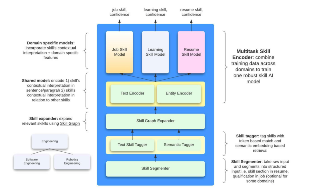 |
|---|
| An overview of the skills extraction architecture |
At a high level, the steps are:
- The Skill Segmenter organizes the raw text into structured input, e.g. a resume is split into the
qualification,career historyetc. sections - The next step aims to generate a candidate list of skills from the context:
- 2a. The Text Skill Tagger is a trie-based model that simply finds matches in the text that exactly match a node in the Skills Taxonomy. This puts the burden on the Skills Taxonomy to have all the aliases that cover every possible utterance of the skill. However, this model is very fast
- 2b. The Semantic Tagger aims to overcome the coverage issues above and uses BERT semantic match to surface more candidates
- 2c. The skills from 2a. and 2b. are expanded into more skills using the Skills Graph. It seems like they add immediate parents, children and siblings of each skill.
- Each skill candidate is scored against the context to generate a confidence score. This section has a Shared Model and Domain-specific Model.
- The Shared Model contains a
context-encoder, which encodes the text surrounding the skill into an embedding, and aentity-encoder, which encodes surrounding skills, the job title, etc. All these embeddings are fed as context into the next stage. The Shared Model assumes that the relationship between the context surrounding each skill and the skill itself is constant across the different domains and thus benefit from a shared module. Their AB tests confirm this hypothesis and show that such multi-task training does increase lift in online metrics. - Each domain (job posting, member profile, course) has its own scoring model. The embeddings from the Shared Model and each skill candidate are fed into the Domain-specific Model, which is presumably a form of cross encoder that generate a confidence score for each skill candidate. Finally, some threshold is applied and a final list of skills is generated.
- The Shared Model contains a
LinkedIn needs to generate skill extractions within 100ms for a high volume of edits. Hence, they used knowledge distillation to distil the BERT model down 80% in parameters.
As we can see, the LinkedIn architecture is fairly complex and context specific. A natural question for smaller players is how we can tap on LLMs today to simplify parts of this architecture to achieve comparable performance.
Hash Collisions
Bloom embeddings is one way of handling large number of user / item IDs. Instead of assigning each unique ID to a unique embedding, we may perform hashing to assign each unique ID to one or multiple bins. The embeddings at these positions are then taken and typically summed to get the final representation of each user / item.
One natural question arises: given n number of unique values and m number of bins, what is the expected number of bins to have 2 or more values assigned to it? This collision is especially a problem if we only represent each unique value with one embedding (i.e. num_hashes = 1). In practice, we would usually have at least 2 or more hashes to avoid this problem.
We may approach the problem by observing that each item is hashed uniformly and has a chance of landing in a particular bin. The hashing is also independent, i.e. it is not affected by the hashing for any other item.
This means that the expected number of items assigned to a particular bin may be modeled as a distribution, since we have n trials and a fixed probability of "success" of 1/m.
- The probability we desire is
- The PMF is , so:
So we may put the above together to obtain . It then remains to get the expected number of colliding bins by , by using the linearity of expectation.
For example, given , the expected number of colliding bins is 1,210 (out of 1 million bins), which is not insignificant.
Now note that since is large and is small, may be well approximated by . Recall that the Poisson PMF is . So:
Using this approximation, we get the expected number of colliding bins as 1,209, which is a very good approximation. Hence the formula we want is:
IMO 2025 Q6
Q6: Consider a 2025×2025 grid of unit squares. Matilda wishes to place on the grid some rectangular tiles, possibly of different sizes, such that each side of every tile lies on a grid line and every unit square is covered by at most one tile.
Determine the minimum number of tiles Matilda needs to place so that each row and each column of the grid has exactly one unit square that is not covered by any tile.
This is an interesting problem with a surprising solution. It's also an easy problem to understand and think about in your head (though certainly not easy to solve!). I have an interactive visualization at https://charleslow.github.io/grid_visualization to explore this problem.
Initial Attempt
The first instinct is to take an approach like below. That is, we observe that using single row / column rectangular tiles is sufficient to tile the grid. Hence the solution uses tiles if the grid is . It's instead of because of the gaps (black squares) up against the grid boundaries. I thought this was the solution initially, and tried to prove it but failed.
My Solution
Let's draw a vertical and horizontal line from each uncovered square (call it a "gap"). Observe there may be 2-4 such lines emanating in the NSEW directions from each gap. Overall, there would be such lines ( because there is no line at the first & last row / column). Let's call each of these lines a "half-line".
Since each row, col pair has one gap, we are assured that a tiling that covers all the half-lines satisfies Matilda (as it will then cover every row and column, except for the gaps).
Now the question is, how quickly can we cover the half-lines with a minimal number of tiles? In other words, how many half-lines can we clear with each tile we introduce?
Now, it is tricky to analyze the number of lines we clear on each turn, because it depends on the preceding steps. For example, if we had cleared all but one remaining tile on each half-line (show example), then the next step can clear a large number of half-lines. It is hard to reason across multiple turns.
So an important observation:
Lemma 1: The number of gaps that each tile touches is an upper bound for the number of half-lines cleared after steps.
Proof. This is quite self-explanatory, as touching a gap is pre-requisite to clearing a half-line that emanates from that side of the gap.
Lemma 1 shifts the analysis from clearing half-lines to analyzing (and maximizing) the number of gaps we touch with every tile we introduce. The number of gaps touched per tile is easier to reason about, as we shall see. We will make the upper bound an equality later on with a specific strategy.
Lemma 2: The number of gaps touched per tile is capped at
4.Proof. This is also not hard to see. Imagine a tile bounded on all sides by gaps. Since there can only be one gap per row and column, the tile cannot be touching more than one gap per side. Since the tile only has 4 sides, it can only touch up to 4 gaps.
4 x 4 Configuration
To get a minimal tiling, we wish to maximize the number of "4-tiles" (i.e. tiles touching 4 holes). This may be done by minimizing the size for a 4-tile at . One such configuration is shown below.
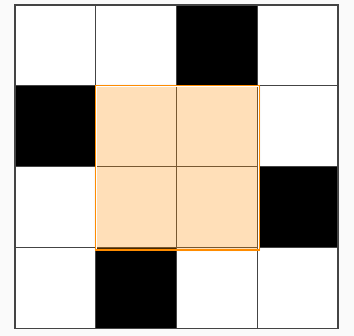
A naive solution is to just replicate this pattern repeatedly along the diagonal, like so. Since we take 5 tiles to tile each mini-grid, this gives us tiles for a grid. For e.g. for a grid shown, the naive solution gives us , but our new strategy gives .
So we already have a lower number than the original naive solution, but can we do better?
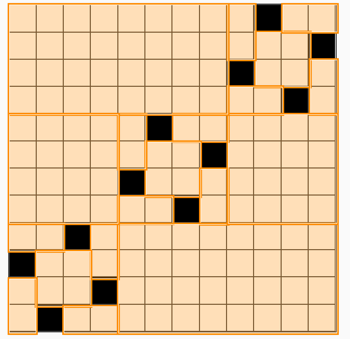
Powers of 4
Staring at the figure above, we can see that putting all our mini-grids along the diagonal is to commit the same mistake as our original naive solution.
More specifically, if we treat each mini-grid as a single square, we can see that the problem reduces once again to the original problem, except that the number of rows and columns shrink by a factor of 4. Therefore, we can squeeze more 4-tiles out by using the same strategy (except that we are now treating each mini-grid as an atomic square).
An example using is shown:
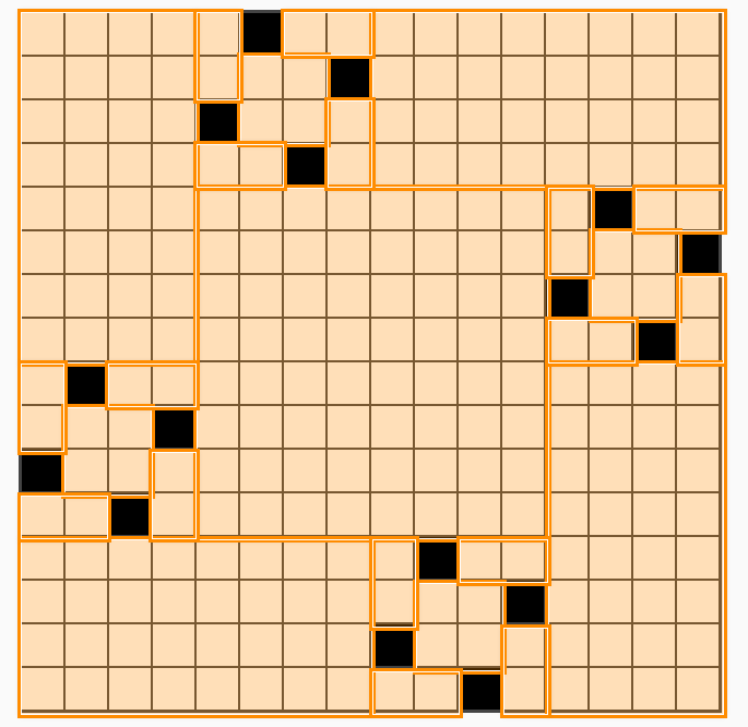
We can recursively use this strategy for grid sizes that are powers of . The minimal number of tiles for a grid of would be given by this recursive formula (for , and ):
Which after expanding gives us the following formula for a grid of :
For example, a grid of requires tiles, a grid of requires tiles, etc.
2025 is not a power of 4
What if our grid is not a power of ? We can split it up into a series of grids that are powers of .
So we create a simple algorithm to do this. Suppose we start with a grid of size .
- At initialization, set our current grid size
- Find the largest such that , and partition out the sub-grid
- Find the minimal number of tiles required for this sub-grid and add it to our current count
- Add tiles to extend the sides to cover the full grid
- Set and continue until
- Use the naive solution for
Applying this algorithm to our original problem of , we have:
So using the formula (and letting to account for the additional tiles for each sub-grid) we have:
Turns out this solution is incorrect. The assumption that the minimum tiling to get a 4-tile turns out to be suboptimal.
Appendix: Code to compute number of tiles
import math
def tiles(k: int):
return int(5 * sum(math.pow(4, i) for i in range(k)))
def largest_power(n: int):
assert n >= 1, "Input must be a positive integer."
k = 0
while 4 ** k <= n:
k += 1
return k - 1
def main(n0: int):
count = 0
n = n0
while n > 0:
k = largest_power(n)
count += tiles(k) + 2
n -= 4 ** k
assert n == 0, f"Remaining value is {n} != 0."
return count
print(main(2025))
Identities
Sigmoid
Sigmoid Relationship to Bradley-Terry Model
Suppose we have scores for objects and . Under the Bradley-Terry model, we can express the preference probability as follows:
Where is the sigmoid function.
Statistics
Adding / Subtracting RVs
Let be two independent random variables. Then .
First, show that where . Proof:
Reference: https://apcentral.collegeboard.org/courses/ap-statistics/classroom-resources/why-variances-add-and-why-it-matters
Summaries of individual papers that I have taken a deeper look into.
Quick Reads
Here I put down quick summaries of papers I read quickly. May possible revisit these with its own page if a deep dive is warranted.
JEPA
Assran 2023 - Self-Supervised Learning from Images with a Joint-Embedding Predictive Architecture
This is the I-JEPA paper. This paper aims to perform JEPA-style self-supervised learning for vision transformers without using image augmentations (like rotation, shear etc.). The main idea is to take a random image patch as context and aim to predict multiple other image patches as target. Importantly:
- The loss is to minimize l2-distance between the and in latent space
- To avoid representation collapse in latent space, the target encoder is updated as a trailing exponential moving average of the Context Encoder
- This approach is simple and scalable and matches performance of SOTA methods using image augmentations
Geng 2022 - Recommendation as Language Processing (RLP): A Unified Pretrain, Personalized Prompt & Predict Paradigm (P5)
This is one of the earliest papers to reframe recommendation task as a language modelling task. The idea is to represent user-item interaction data and other metadata in recommendation tasks as an input to response task for supervised fine-tuning (or pre-training). Then we can have a unified language model to perform various tasks in a recommendation system.
The tasks proposed are:
- Sequential Recommendation: Given purchase history
item_123, item_456, what is the next item?1581 - Rating Prediction: What star rating would
user_123give toitem_456? 5.0 - Explanation Generation: What explanation or review would
user_123give toitem_456(iphone case)? You can use it to protect your phone - Review Summarization: Give a short sentence summarizing this review
<insert review>.<insert summary> - Direct recommedation: Pick the most suitable item from the following list to recommend to
user_123:item_123, item_456, ....item123
These tasks are mixed together and then used to pretrain an encoder-decoder model from scratch, and then used for various recommendation tasks.
Tang 2023 - SE-DSI
This is an expansion of the Differentiable Search Index paper. The argument is that teaching an LLM to learn arbitrary document ids is not semantic. Hence we should represent documents as semantic words to aid learning.
Specifically:
- Docid Representation. For each document, use a T5 model to generate a query to serve as document identifier (5% collision).
- Input features. Use 3 types of input features to predict the "query docid":
- Whole document
- Key passages identified using textrank
- Key sentenes identified using textrank
This approach beats vanilla DSI, as we use semantic information as document representation. Note that evaluation task is Q&A.
Chen 2023 - Understanding DSI for Text Retrieval
Analyzes the shortcomings of DSI through 3 metrics:
- Exclusivity: There should be a one-to-one mapping between document contents and semantic ID.
Task: Given first N tokens of document, can we retrieve the correct ID
- Completeness: The LLM should remember as much information about each document as possible.
Task: Use BERT model to find important chunks in document, then use these chunks as query to see if we can retrieve the correct ID.
- Relevance: Can the LLM rank documents in relevance order to a query.
Task: For a given query, check the document at positionkof the LLM's recommendation order to see how relevant it is. Specifically, measure the cross encoder score of document against the query and compare to score of a random document . Lower score is considered a failure- Found that DSI only generates relevant documents at position
1, and then becomes highly irrelevant thereafter.
Proposed improvements:
- Data Filtering: Break each document into chunks and use a teacher model
TCT-Colbertto perform retrieval using that chunk as query. Only successful retrievals that get the document back are considered useful content used for LLM fine-tuning. - Multi-task learning: Normal DSI indexing task only seeks to predict one document ID given its contents or a query. They propose to add an additional task where we get LLM to learn to predict a list of relevant document IDs.
- The list of relevant document IDs are generated using a teacher model (
TCT-Colbertagain).
- The list of relevant document IDs are generated using a teacher model (
Ju 2025 - GRID
Snap's GRID repository which is a modular repo for semantic ID based generative retrieval to facilitate architecture comparison. A generative retrieval system has the following components:
- Semantic ID Tokenization:
- Convert item description to embedding
- Quantize embedding to tokens (K-means, VQ-VAE, RQ-VAE)
- Sequential Recommender:
- Whether to use user token
- Data augmentation using sliding windows
- Architecture: Encoder-decoder vs decoder only
- Beam search
Note: this system only considers the case where each user is represented as a sequence of items, and the LLM is trained from scratch (not finetuned from pretrained).
Their experiments are interesting:
- Residual K-means tokenization is best, compared to VQ-VAE and RQ-VAE. This is quite surprising and I'm not 100% convinced.
- Larger OTS embedding models are better, no surprise.
- Encoder-decoder sequential recommender is clearly better. Somewhat surprising, I guess there is some inductive bias that is useful in this setting to have full attention over the user sequence.
- Sliding window is better. Sliding window means that given a training data sequence of a user represented by item interactions, we generate all possible contiguous sequences to augment our dataset. Not surprising.
- SID de-duplication is unnecessary. Between appending an arbitrary token to deduplicate SIDs or just randomly selecting from SIDs with multiple items hashed to it, the performance difference is negligible. This is assuring that we don't need to further complicate the system.
- Constrained beam search is unnecessary. Constrained beam search means that we maintain a trie to only generate tokens leading to a valid SID. The results show that this has negligible performance difference to unconstrained beam search, which has much better efficiency. This is assuring that we can just use uncontrained beam search.
Weinberger 2009 - Hashing for Multitask Learning
Weinberger 2009 - Feature Hashing for Large Scale Multitask Learning
This paper proposes a method to represent a large feature set in a smaller space by using hashing. It shows analytically that with a sufficiently large hash dimension :
- The inner product between instances is preserved, i.e. doing a dot product between instances in the hashed dimension approximates the true dot product in the original dimension
- The same applies to learning a weight vector to generate predictions in the hashed space: the error of approximation goes to zero as increases
Setup
Consider having data points , where can be very large (e.g. millions). This setting is easily realized when we use, for example, word bi-grams and tri-grams as term-frequency features to perform some kind of text classification task. Such a large feature vector is unwieldy, and also inefficient since the feature vector is very sparse for a given text.
The hashing trick maps the high dimensional input vector to a smaller dimension feature space with the notation , such that .
We start with the following definitions:
- Let be a hash function
- Let be a hash function
Note that while the definitions map from an input integer, we may apply them to texts as well, since any finite-length text may be assigned to a unique integer. This is typically done in practice by applying some hash algorithm to a given string, and then using the modulo function to restrict it to the desired range.
With this, and given two vectors , we define the hash feature map:
Where is an index in the hashed dimension space, and is an index in the input dimension space. We get a hash collision if more than one term is hashed into a given position . For brevity, we may just write .
Analysis
With this setup, the paper aims to prove analytically that hashing in this manner preserves the characteristics of the original space. In other words, we can significantly reduce the dimension of our features but achieve the same predictive effect as the original space by doing the hashing trick. This also means that the detrimental effect of hash collisions is minimal with a sufficiently large .
We won't trace through all the results, just the important and simple ones.
Lemma 2 The hash kernel is unbiased, i.e. .
Proof. The proof simply starts by expanding the inner product in the hashed space as follows:
Where is an indicator variable which takes if (i.e. they are hashed to the same position) and otherwise.
To see that this expansion is true, consider a position in the hashed space, e.g. . The value at position looks something like the following. We just need to move the summands to the left and use the variable to denote the common hash positions where and interact (if i and j are hashed to different positions, they clearly do not interact in an inner product).
Now note that we can decompose the expectation over into its independent constituents, i.e. and respectively (since the two hashes are independent):
Now we just need to observe that the hashed values are independent from all other terms in general, but also independent from each other whenever (provided our hash function is pairwise independent). Thus when , the summand is:
These are clearly because . So the original summation reduces to:
Not only is the hashed inner product unbiased, it also has a variance that scales down in . The proof does a similar but more tedious expansion as the above, and assumes that have l2-norm of . This suggests that the hashed inner product will be concentrated within of the true value.
These results are sufficient to justify use of the hashed inner product space in practice. That is, we can perform recommendations in the hashed space with sufficiently large (we can tune that using validation error) to make the large feature space tractable. The paper goes on to prove more detailed bounds on the error and norm which are of less practical significance.
Multi-task Learning
The authors argue that this method is especially useful in the multi-task learning setting. Consider an email spam classification task where the vocab space is and the user space is . The parameter space is thus , i.e. we wish to learn a user-specific weight vector for each user , which allows us to personalize the spam filter for each user (different users have slightly differing definitions of what is spam).
The authors suggest the following approach:
- Use the hashing trick to hash each term into the hashed space. e.g.
datais passed into a global hash function and assigned to a position - Each user gets his/her own hash function . This may be implemented by using the same hash function but appending the
user_idlike so:user1_data, which hashes the same term into a new position. - We may thus represent each instance by , capturing both a global element (some terms are universally spam-indicative) and a personalized element (some terms are specifically indicative for a user)
- Finally, we learn a weight parameter by training it in the hashed space
Empirically, for their task of , , they found that performance starts to saturate with . This is a very small fraction of the total space , showing the effectiveness of their method. Nevertheless, we should note that 4 million is still a rather large space.
Rendle 2009 - Bayesian Personalized Ranking
BPR: Bayesian Personalized Ranking from Implicit Feedback
This is one of the most cited papers for collaborative filtering. It proposes a pairwise learning algorithm for item recommendation from implicit feedback that remains one of the most performant to date. It is pitched as a rival method to Weighted Matrix Factorization, the other strong model of the day. BPR argues that it is superior to WMF because it explicitly optimizes for ranking.
Setup
Let , denote the set of all users and items respectively. We have access to an implicit feedback data . The task is to produce each user with a personalized ranking . Note that denotes the cartesian product of with itself, so it represents the set of all ordered pairs of elements of . The ordering is a subset of these pairs where a preference relationship is indicated by the model. For convenience we also denote:
In implicit feedback systems, only positive interactions between user and item and observed. The typical approach is to put the interactions in a matrix and fill in unobserved entries with . A model is then fitted to this model. The paper makes an interesting observation that this problem is ill-defined, since a perfectly expressive model that fits the training data perfectly will fail to make any prediction at all, since all unobserved entries will be given a score of . Hence regularization methods are employed to avoid such overfitting.
The idea of BPR is to avoid making judgment on the pairwise preference between two items with the same score. That is, if items and are both interacted by user , we cannot judge if one is preferred over the other. Also, if and are both unobserved interactions, we cannot make such judgement either. Thus the training data is denoted by the following.
Note that this definition means that , since cannot be positive for if it was included as a negative.
BPR Loss
The bayesian formulation for finding a ranking is to find the model parameters that maximize the following probability:
We assume that:
- All users act independently of each other
- The ordering of each pair of items for a given user is independent of the ordering of every other pair
Then, we can write the likelihood across all users as: Where is the indicator function for the preference relationship. In other words, the likelihood of the overall ordering is the product of the likelihood of each triplet. For each triplet, the likelihood is given by the model's prediction for given label or .
Note that the above term is only not equals to if or . Also, since we observed above that and vice versa, only one of the two terms will come into play for each entry. The above formula can be simplified to:
Note: Not too sure about the above step, would have thought that the term should also come into play when .
Model
Now we can model the preference probability using a model as: Where denotes a BPR-agnostic model that generates a predicted real-valued score for the triplet . Note that is the sigmoid function.
To complete the bayesian modelling, a prior distribution is introduced over the model parameters. For simplicity, we let take the form of a multivariate normal distribution with zero-mean and all covariances zero, with equal variance for each parameter (i.e. ):
The maximum posterior estimator for is thus given by the following:
Note that in the last step, the log prior is translated into L2 regularization. This is apparently well studied and I will explore the derivation at a later time. A possible resource is Yuki Shizuya - Understanding L1 and L2 regularization with analytical and probabilistic views.
The paper suggests using SGD updates (i.e. batch size of 1) by randomly sampling triplets with replacement from . This converges much faster than doing user-wise SGD.
Finally, we've assumed is model-agnostic up to now. For matrix factorization, the authors suggest the following form. In other words, we compute the prediction for each user, item pair (usually via dot product of embeddings, but can be anything) and take the difference.
Cornac Implementation
Cornac has a Cython implementation of BPR that is fast (but not memory scalable when number of user and items is large). num_threads can be increased for faster parallel processing (Cython overrides the GIL).
At initialization:
- User embedding
Uof shapen_users, kis drawn randomly from a standard uniform distribution wherekis the embedding dimension - Then, we take . I suppose this leads to small, centered values which leads to stable initial training. Normalizing by
kensures that the dot product between vectors does not explode. - Item embedding of shape
n_items, kis initialized similarly - Optional bias vector of shape
n_itemsis initialized to the zero vector
Note that train_set.X is a scipy.sparse.csr_matrix, which has 3 main vectors:
data: values of non-zero entriesindices: column indices of the non-zero valuesindptr: index pointers to the start of each row indataandindices
The vector user_ids is constructed from the csr_matrix. It is of the same length as X.indices and represents the row indices of the non-zero values. Thus we have both row and column indices of the non-zero values.
The main training loop samples a (u, i, j) triplet randomly each turn. It does so by the following steps:
- A random index
ibetween0andlen(user_ids)is generated - The
user_idanditem_i_idare obtained by indexinguser_ids[i]andX.indices[i]respectively - Now a random index
jbetween0andn_itemsis generated - The
item_j_idis obtained by indexingneg_item_ids[j]whereneg_item_ids = np.arange(n_items) - A check is performed on the sparse matrix that
item_j_idis not a positive item foruser_id. If so, we skip this triplet. - Pointers to the start of the relevant
u, i, jembeddings are then obtained - Note that
1epoch compriseslen(user_ids)number of triplets
The Cython code then computes and manually applies the SGD updates derived in the paper. Will omit since we do not need to manually compute the updates if using autograd.
Note: This implementation of BPR assumes binary relevance (an item is interacted or not). It does not allow for finer-grained preference relationships (e.g. a floating point rating score to rank items), which in theory BPR does support.
From RankNET LambdaRank LambdaMART
This is an overview paper that explains the model behind LambdaMART, a technique used to learn Gradient Boosted Trees that optimize for NDCG on recommendation-type of datasets.
RankNET
RankNET is a generic framework for training a learn to rank model. Given a differentiable model that produces a score from an n-dimensional input vector, RankNET is able to train such that for a given query session with items and corresponding features , learns to predict the relationship for any two items in the query session when is a better recommendation than . The differentiable model is typically a neural network or boosted trees.
RankNET uses revealed pair-wise preferences within each query session to train . Specifically, suppose we have a data for one query session as follows:
| query | item | clicked |
|---|---|---|
| qid1 | a | 0 |
| qid1 | b | 1 |
| qid1 | c | 0 |
We can transform this data into a pairwise dataset as follows, where denotes the preference relationship between and which we inferred from the click data. Note that the pairwise comparisons are only made within the same query session (e.g. qid1), as it reflects a given user's preferences in the context of a query and the items impressed to him/her in that session.
| query | |||
|---|---|---|---|
| qid1 | a | b | -1 |
| qid1 | a | c | 0 |
| qid1 | b | a | 1 |
| qid1 | b | c | 0 |
The pairwise setting is now more amenable to modelling (compared to directly optimizing for a good ranking), since we can now treat the task as a classification problem. For each row of the pairwise dataset, we only need to model the probability that is preferred (or not) to . This can be formalized using a cross entropy loss comparing the predicted preference of our model to the revealed preference in the dataset.
First, we model the predicted probability from the model. Given row of the pairwise dataset and and respectively, we model the predicted probability that is preferred to (using to denote a preference relationship) by passing the score difference between the predicted scores and for items j and k respectively through a sigmoid function, like so:
Now let us denote the revealed probability that is preferred to as such that:
- if we prefer item j to item k
- if we have no preference between the two items
- if we prefer item k to item j
The cross entropy loss of our model can then be expressed as:
For convenience, let us denote (and conversely, ), which translates into the following:
- if we prefer item j to item k
- if we have no preference between the two items
- if we prefer item k to item j
Let us also define the convenience variable . The cross entropy loss then simplifies to:
Note that in line 2 of the above, we use the useful identity that and . In line 3, the first and last term of line 2 cancel out to simply return .
Having written out the loss function, we now need to differentiate the loss with respect to the model scores and parameters to obtain the gradient descent formula used to train the RankNET model. Differentiating wrt and gives:
Note that the first line of the above uses the result . We obtain line 2 by multiplying the right term by in both the numerator and denominator. We obtain line 3 by observing that is a function of , such that and likewise . The symmetry of the derivative wrt and will be important for the next section on factorizing RankNET to speed it up.
Finally, we use the gradient to update individual parameters of the model . In the below, denotes the number of data points in the pairwise dataset. This update procedure rounds up the discussion on RankNET and is sufficient for training a generic differentiable model from ranking data.
Factorizing RankNET
Schroff 2015 - FaceNET
Schroff 2015 - FaceNet: A Unified Embedding for Face Recognition and Clustering
This paper proposes the Triplet Loss for learning a face recognition system.
The task is that given a large number of person identities with a number of images associated with each person, to learn a model representation for an image in euclidean space, such that images belonging to the same person are close by and images for different persons are far away. This paper was impactful because it improved the SOTA on face verification by a large margin.
At this point, representation learning often trained a CNN classification model to classify images to a known identity. A bottleneck layer of relatively low dimensionality in the middle of the network is chosen as the representation of an image. In contrast to this indirect method, this paper directly optimizes the representation using contrastive learning.
Setup
Let the embedding of image be represented by , and constrain . Now for a given person i, we want the anchor image to be closer to other images of the same person (positive) than images of any other person (negative), with some margin . That is, we desire a model such that:
Where denotes the set of all possible triplets in the dataset. The authors note that most triplets would easily satisfy the desired constraint, hence we need some way to picking good triplets to optimize the learning process.
The loss we desire to minimize is thus as below. The intuition is that we want the anchor-positive distance to be small but the anchor-negative distance to be small.
With this loss function, we see that we have 3 types of triplets:
- Easy triplets where . These will contribute 0 loss since will be a negative value, and the positive operator makes the loss 0. This makes sense because the model already categorizes these triplets well and there is nothing more to learn from these examples.
- Semi-hard triplets where . These will contribute a small loss, since . These are triplets where the positive is already closer to the anchor than the negative (which is good), but the distance is still within the margin so we want to make the distance greater. In other words, .
- Hard triplets where . These will contribute a large loss. These are triplets where the negative is closer to the anchor than the negative.
Triplet Selection
As with most contrastive learning methods, the authors observe that the selection of triplets is important for learning well. In an ideal world, we would want to select the hardest negatives for each anchor, i.e.:
However, this is undesirable because:
- We may end up mostly selecting mislabelled instances or corrupted images
- It is computationally infeasible to search across the whole corpus
- Trying to learn hard negatives at the start of training may cause learning to collapse
Hence, the authors propose:
-
Mini batch negatives. Instead of finding the hardest negatives across the entire corpus, they mine for the hardest negatives in the mini-batch. This improves computational efficiency and mitigates the mislabelled/corrupted data issue.
-
Curriculum Learning. At the start of training, the authors select easier triplets, and gradually increase the difficulty as training goes along. Presumably, this is done by thresholding negatives based on and starting from high to low .
-
Semi-hard negatives. The authors mention that it is helpful to limit negatives to , but it is unclear whether they always do this or only at the start of training. The intuition is to cap the difficulty of the triplets, as triplets that are too difficult may actually hinder learning due to corrupted data or mislabelling.
Note: In a later paper Lee 2020 - Large Scale Video Representation Learning via Relational Graph Clustering, it implies that FaceNET uses semi-hard negatives throughout the entire training process, which makes sense given that the paper warns against using hard negatives. In light of this, I would presume FaceNET searches for the hardest semi-hard negatives in each mini batch as negatives for each triplet.
Application to Semantic Search
The triplet loss may be applied directly to semantic search. However, it is important to note that the paper assumes that for each person, all others-labelled instances are negatives. This is a suitable assumption for face recognition as each image can only belong to one person, but it is not true for semantic search, where a document may be relevant for multiple queries. Hence, the mislabelling issue when mining hard negatives is amplified for semantic search. I imagine that the selection of accurate negatives for semantic search would require more verification and filtering.
Covington 2016 - Deep NNs for Youtube Recs
Deep Neural Networks for YouTube Recommendations
This is an old paper that documents YouTube's recommender system, but quite foundational in the Recsys world. This paper also occurs at a time when there was a migration of models into deep learning methods, and Tensorflow was open sourced in the year before.
Retrieval
As with most recommender systems, there is a candidate generation and ranking step. The candidate generation surfaces "hundreds" of videos. The predecessor to this work is a matrix factorization approach trained under rank loss (assuming it is BPR). This work may be thought of as generalizing the MF approach to non-linear transformations of arbitrary features.
The paper views recommendation as an extreme multiclass classification problem, where the aim is to predict the probability that the video watch at time is video . In the below, is the corpus of videos, is a specific user and is a specific context. Also are high dimensional embeddings representing user and item respectively.
It is well known that the above is intractable with millions of classes, so this paper samples negative classes from the background distribution and then corrects for the sampling via importance weighting. This paper samples "several thousands of negatives" for each true label, and then minimizes the softmax loss for the true label against the negatives. Note: it is not specified what is the background distribution, it could either be a uniform distribution over items or the empirical marginalized impression probability of each item over a fixed time period. Also note that the modern approach is to use in-batch negatives for efficiency, as opposed to the purely random negatives approach here.
At serving time, a fast ANN search algorithm is used to find the top scoring items. This paper used a hashing algorithm in Weston 2013 - Label Partitioning for Sublinear Ranking for this, which is probably an outdated approach today.
Retrieval: Features
Each user is represented by features such as:
- Watch history, represented by a variable-length sequence of video IDs. Each video is represented by an embedding, and then the element-wise average is taken such that the whole history is represented by a dense embedding. Note: this is prior to the attention mechanism, the modern approach is to run the sequence through self attention before taking the element-wise average to get a more nuanced representation.
- Search history, represented by a variable-length sequence of search terms, treated similarly to watch history. Note that in the experiments, both watch and search history were capped at
50terms each. - Categorical features such as Geographic location are embedded into a dense vector.
- Simple binary and float features such as gender, log in status are input directly into the network as real values normalized to [0, 1].
The features are all concatenated together to form a long dense vector representing the raw user inputs. e.g. if watch and search history are length , concatenating would give a vector of and so on. The dense vector is passed into a fully connected feed forward network with shrinking layers to get a final fixed size dense vector representing the user. Similar approach is done for items.
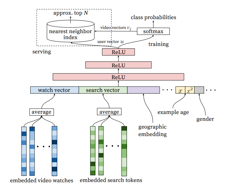 |
|---|
| Candidate Retrieval Architecture |
Retrieval: Example Age Feature
Since video popularity typically spikes in the first few days after upload and dies down after, an important feature is the "example age" to capture the "freshness" of an item. Since we typically have a training window of several weeks, failing to account for the age of an item would mean that the model will learn to predict the average watch probability of a video over the entire training period. This is not ideal since it makes the model biased toward older videos (which have had more time for exposure) than newer videos.
The authors correct for this by including the age of the training example as a feature during training. Suppose our training window is 90 days, then this feature would range from 90 (or 1 after normalization) for training examples on the first day of the training window to 0 for training examples on the last day of the training window. At serving time, the value of this feature is set to 0 to reflect the fact that we are making predictions at the very end of the window. The authors show that this approach helps the model learn to predict the time-sensitive effect of popularity for a given item that matches the distribution in the data.
Note: This is different from incorporating the age of the item as a feature during training. I suppose while age of the item can capture the same information, it requires more work at serving time, since we need to set the feature value to the actual age of the item at the time of serving. In contrast, the above approach allows us to just set the feature to 0 which is more elegant.
Retrieval: Surrogate Problem
The paper emphasizes that recommendation involves solving a surrogate problem that is then transferred to live inference. Hence care must be taken to ensure that we do not overfit the surrogate problem which can hurt live metrics. Some insights are:
- Generate training examples from all YouTube video watches, not just from YouTube's recommendations, so that relevant videos can be propagated quickly even if they did not originate on YouTube itself.
- Generate a fixed number of training examples per user, so that very active users do not dominate the loss function. Not sure how this works in practice, presumably a fixed number of examples per user (or just 1?) is sampled for each training epoch. This significantly improved live metrics.
- Withhold information from the classifier. This is a counter-intuitive point that shows us how tricky it is to find a good surrogate problem. Given the structure of YouTube, users can find videos either from homepage recommendations or from searching for a video. In the latter case, if a user searches for say
taylor swift, it is typically followed by user watches oftaylor swiftvideos. However, we do not want to reproduce this behaviour for homepage recommendations, such that a user is always shown search results based on his / her last search query - this would perform very poorly! Hence the representation of search terms using a simple element-wise average (instead of using a sequence model like RNNs) actually leads to better live results. - Predict the next watched video. It is important that training is not performed on random held-out samples, but that the next video is always held out and a "rollback" of features available prior to the video watch is supplied to the classifier. This is because video watching is highly sequential in nature, e.g. episodic videos are watched in sequence and users explore artists starting with the popular videos before moving to niche ones, hence it is important that the surrogate problem captures this behaviour.
Retrieval: Ablation Studies
The paper explored a few settings. At depth 0, the MLP simply transforms the dense input vector in one step to the output dimension of 256, i.e. essentially a linear approach. For depth 1, an in-between ReLU layer of 256 is introduced; for depth 2 in-between ReLU layers of 512 -> 256 is introduced and so on. The performance increases significantly from depth 0 to depth 1 with diminishing benefits as we increase the model size.
In terms of features, it is interesting that incorporating searches is very important for performance.
Watches onlyhas MAP of around 6%Watches + Searcheshas MAP of around 9%Watches + Searches + Example Agehas MAP of around 10%All featureshas MAP of around 11%
Ranking
The difference between ranking and retrieval is that ranking aims to specialize predictions to the specific setting in which impressions are shown. In practice, this means that the ranker has access to many more variables about the video and the user's relationship to the video than the retriever. The general architecture for the ranking model is similar to the retrieval model, with the difference that the impressed video is also included as part of the features and the model simply outputs a logit for prediction.
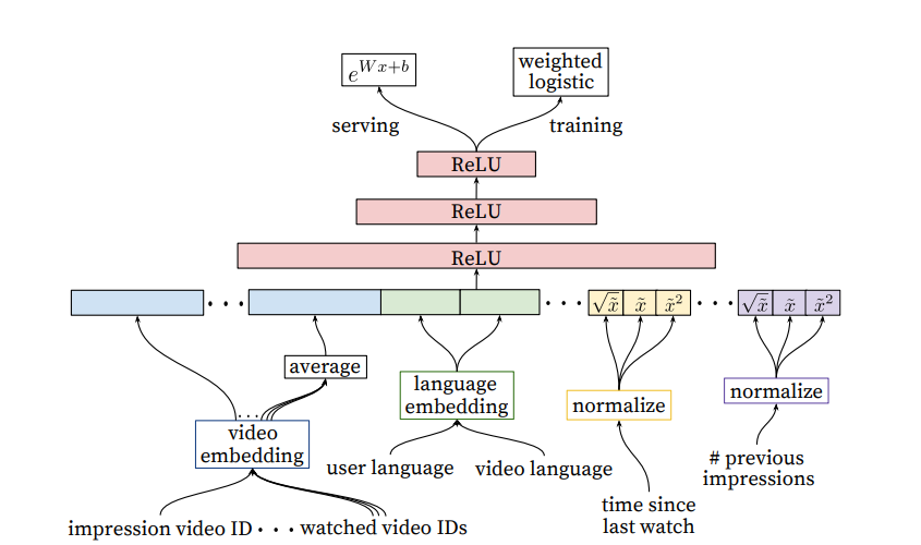 |
|---|
| Ranking Architecture |
Ranking: Feature Engineering
Despite the promise of deep learning, this paper found that significant time was still spent engineering features due to the challenge of encoding features for recommender systems. The main challenge for the authors was in representing a sequence of temporal user interactions and how these actions relate to the video being impressed. Note: The modern approach seems to move away from such intense feature engineering. Instead, the past interactions and video being impressed are simply embedded and passed into a self attention mechanism. The model can then learn interaction features in the hidden layers. The downside of the modern approach is paying higher compute cost at inference time, but it may still be worthwhile given the significant engineering effort required for generating and retrieving hundreds of features manually.
The paper highlighted User-item previous interaction features as the most important and impactful. This includes features such as:
-
How many videos from this channel did the user watch before?
-
When was the last time the user watched a video on this topic? These continuous features describing past user interactions on related items are especially powerful
-
Features describing number of past impressions of this (user, item) pair are important for a responsive recommender system. For example, if the user was shown this item many times recently but did not interact with it, the recommender can learn to demote this item so that the user's recommendations can be "refreshed".
Note: For YouTube, they maintain such impression features at up-to-the-second latency because of its importance. For other use cases, a latency of say 15 minutes might still be quite helpful.
-
Feature scores from candidate generation step are also useful
Similar to the retrieval step, categorical features are represented by dense embeddings, with a separate embedding table per categorical feature. The vocabulary for each feature is determined by a single pass over the training data at training time, and the vocabulary size is capped at 1 million based on impression count. Out of vocabulary values during inference time are simply mapped to the zero embedding. Multivalent features (e.g. a sequence of video IDs for watch history) are averaged element-wise before being concatenated.
The paper also found that normalizing continuous features was critical for performance. Specifically, a feature value with empirical distribution will be normalized to , which is the cumulative probability of the empirical distribution up to value . To make it tractable, the authors compute the quantiles of the empirical distribution and do linear interpolation between the quantiles. For e.g. if the empirical distribution of is (1, 2, 8, 10), then 1 will be mapped to 0.25, 2 to 0.5 and so on. Note: this is different from min max normalization, which only uses the min and max value.
Ranking: Predicting Watch Time
The authors found that predicting watch time instead of a binary watch variable gets much better performance at live metrics. This is incorporated into the model in the form of weighted logistic regression. For positive examples (where the user did watch the video), the example is weighted by the amount of time the user spent watching the video. For negative examples (where the user did not watch), the example gets unit weight.
Recommendations as Treatments
Training and evaluation data for recommender systems is subject to selection bias, because the probability of observing a data point depends on (i) users interacting with items which they like and (ii) the recommender system pushing items which they think the user likes. This leads to data Missing Not at Random (MNAR) and leads to biased model training and evaluation.
Consider users interacting with movies. Denote users and movies . Let denote the true rating / interaction matrix between user and item, and the predicted matrix. Let be the observability matrix of whether an interaction was observed, and be the probability of observation, i.e. . Ideally, we want the propensity matrix P to be uniform across all entries, which gives us the Missing Completely at Random (MCAR) condition.
Evaluating only on observed entries is biased
Given a model , we often want to compute evaluation metrics on how well approximates . For example:
The Risk function may then be denoted:
However, cannot be computed because most entries in are missing. Typically, we estimate using only observed entries. This estimator is naive because it simply assumes the propensity matrix is uniform. This assumption is often false in recommender systems because a small set of popular items tend to get impressed a lot. Hence this estimator will favour models that lean towards the popular items compared to models that recommend rarer / new items.
Unbiased estimators
The main idea in this paper is to view this problem as analogous to estimating treatment effects in causal inference. Think of recommending an item as an intervention analogous to treating a patient with a specific drug. The goal is to estimate the outcome of a new recommendation (clicked or not) or new treatment (recovered or not), while most outcomes between u,i pairs are not known.
The key to resolving this bias is to understand the assignment mechanism that generated , namely the propensity matrix . We can then correct for the propensity. We need to assume that , i.e. full support, because otherwise the IPS estimator below is undefined.
IPS Estimator
The main estimator is the Inverse Propensity Score (IPS) estimator. Assuming that the assignment mechanism is known:
We have simply normalized each score by its inverse propensity, so that popular items with a high chance of being shown get their score reduced proportionally (and likewise in the opposite direction for rare items).
We can show that the IPS estimator is unbiased as we take the expectation over the random observability matrix. That is, suppose we are allowed to sample an infinitely large number of observations based on , the average of the IPS estimator over these datasets will be the true risk function. This simply happens because the expected value of is simply the propensity, and if we know the propensity we can just cancel it out.
Comments
- This paper only addresses exposure bias, but not position bias. In other words, it assumes that all impressions are equal, which is valid when a user is shown an ad, but not when a user is shown a list of search results. In the latter case, items in lower positions have a lower probability of being considered by the user, even though both are considered to be observed.
Doersch 2016 - Tutorial on VAEs
Tutorial on Variational Autoencoders
Tutorial on VAEs from a computer vision perspective.
Introduction
Generative modelling deals with models of distributions , defined over data points . For example, may represent pixels of an image. may indicate that a set of pixels that look like a real image has high probability, whereas images looking like random noise get low probability.
For generative modelling to be useful, we don't just want an unconditional distribution. Instead, we want to generate images from a conditional distribution, e.g. images that look like another image or following a certain caption.
Latent Variable Models
Generative modelling usually starts with a latent variable. For example, in digit image generation, we may first want to choose a particular digit (say 5) to generate. The image model then knows to generate pixels corresponding to this digit (as opposed to deciding on the fly). is typically chosen to indicate the latent variable (which can be multi-dimensional).
Formally, we have a vector of latent variables which we can easily sample from based on some probability density function defined over . In VAEs, this distribution is typically a multi-variate standard gaussian distribution.
We now want to make sure that we have some function that maps from the latent variable space to the output space . Say we have a family of deterministic functions (typically some neural network) which is parametrized by a vector , where . In this setup, randomness is injected by the random variable such that is a random variable in the space .
To actually generate images that look like , we wish to optimize such that we can sample from and with high probability, will look like that 's in our data.
How do we formalize this notion? Naively, just gives a random point prediction. We need some probability distribution which tells us how likely a given training sample is under the generative model . By the law of total probability, we can then write down the Maximum Likelihood objective:
The choice of for VAEs is often gaussian. Specifically, the most standard choice is:
This means that the function gives us the gaussian mean, and the covariance matrix is a fixed diagonal (as is a hyperparameter). Notice that this gaussian expression allows us to express the idea that we just need to produce samples that look like , but does not have to exactly match some .
This smoothness is critical for generative modelling — if we specify to be the dirac delta function (i.e. all the probability mass is on the specific output produced by ), it would be impossible to learn from data, as the function is zero almost everywhere.
Also note that while gaussian is the most common choice, it does not have to be so. We just need to be computable and be continuous in . For example, if is binary, then can be a bernoulli parametrized by (although it's unfathomable why one would do this).
Variational Autoencoders
In order to maximize above, there are two big problems to solve:
- How do we define the latent variables and what information they encode
- How to deal with the integral over
Problem 1: How to represent Latents?
For the first problem, VAEs basically prescribe minimal structure to the latents , and say that the samples of can be drawn from a simple distribution, say . Then, the onus falls on the model to map from a simple gaussian distribution to the complex distribution which describes our data. We know empirically that this is not a problem for an arbitrarily large neural network.
Problem 2: How to deal with integral over P(z)?
For the second problem, the naive approach is to deal with the integral via sampling. That is we sample a large number of latents and compute . The problem with this approach is that in high dimensional spaces, we need a very large to get an accurate estimate of . This is because for most instances of , will be very close to .
The key idea behind VAEs is to speed up sampling by attempting to sample values of that are likely to have produced , and compute just from those. To do this, we need a new function which when given an image , produces a distribution over values likely to have produced . If the space of values that are likely under is smaller than the space of values that are likely under , we will be able to estimate much more cheaply.
However, by introducing a new arbitrary distribution , we are no longer sampling under , so we cannot directly obtain from it. Thus we need some way to relate and . This relationship is one of the cornerstones of variational Bayesian methods.
Let us start by defining KL divergence between and some arbitrary distribution (which may or may not depend on ).
Recall that KL divergence is asymmetric, and measures how different two probability distributions are. In this case, the expectation is taken over the distribution of values under .
Now apply Bayes rule to , and do some rearranging:
Some comments on the above:
- comes out as a constant because it does not depend on .
- We can group and together into its own KL divergence term.
So far, we have not made any assumption on the arbitrary distribution . In the context of trying to maximize , it makes sense to construct a which does depend on . So we make that dependency on explicit. Let's call this the ELBO equation.
This equation is core to the VAE, so we should understand it deeply.
- The left hand side represents what we want to optimize:
- was the original maximum likelihood objective - we want our model to produce images that look like
- is the error or deviation of our tractable, estimated distribution from the true, intractable oracle distribution . This term is always more than or equals to and is if and only if .
- The right hand side is called the Evidence Lower Bound (ELBO). In bayesian statistics, the marginal is called the evidence, because our data is evidence for how good our model is. The RHS is a lower bound for our evidence precisely because the KL divergence term , which implies .
- We cannot directly optimize , but we can do the next best thing which is to optimize the tractable RHS, given an appropriate choice of .
- As we increase the capacity of , the "error" term should become smaller and smaller, so the RHS will more accurately estimate the evidence (and lead to better optimization)
Notice how the RHS now resembles an auto-encoder:
- "encodes" into a latent
- "decodes" back to reconstruct
Optimizing the Objective
Now we need to perform SGD on the RHS. First we need to specify . The usual choice is:
Where and are both neural networks with parameters that map a given deterministically into a mean and variance vector respectively. We only need a vector for the variance because is typically constrained to be a diagonal matrix.
Because we chose both to be multi-variate gaussians, the KL divergence between them may now be computed in closed form ( is the dimensionality of the distribution):
The second line above gives the general case, but since our , it reduces into the third line. The functions express the fact that the parameters of the normal distribution of are determined by .
Reparametrization Trick
So we have the second term on the RHS expressed as a function of , which can be optimized via SGD. What about the first term ?
This term is more tricky, because it involves two steps. Suppose we approximate the expectation by performing SGD. Then we have to:
- Sample a
- Compute using the decoder
The first sampling step is not an operation that can be backpropagated through, so we cannot optimize this equation as-is. This is where the re-parametrization trick comes into play.
The re-parametrization trick essentially moves the stochasticity of the sampling step out of the model forward pass into the data layer. Instead of sampling directly, we first sample an intermediate and treat it as data. Then, we compute deterministically . This achieves the same effect as the direct sampling approach, but the difference is that the parameters of have entered the equation in a deterministic way that can be backpropagated.
With the trick, we now have fully specified the optimization objective. The equation we take the gradient of is:
On the second term :
- Note that we have already spelt out the closed form expression above, which involves the encoder neural networks .
On the first term :
- This is the reconstruction loss which measures how well we reconstructed the input after passing it through the encoder back to the decoder again, so it involves both the encoder and decoder.
- Specifically, we first sample an , then compute , which gives us one sample of an encoded input .
- Recall above that we specified , which is a PDF of a normal distribution with mean given by the decoder applied to sample and some constant variance.
- Hence which is an l2 distance
Test Time Inference
At test time, when we want to generate new samples, we simply sample a new , then feed it into the decoder to get a new .
Suppose we want to evaluate the probability of this new test example, i.e. . This is not tractable for the reasons we discussed earlier, as it involves an integral over the distribution of . However, we can make use of the ELBO concept and use the RHS of the ELBO equation as an approximation to . There is still an expectation over , but because sampling gives an expectation that converges much faster than sampling , we can get a good sense of the probability by sampling a few times.
Extra Info
This section tackles 3 questions to help our understanding:
- How much error is introduced by the additional term ?
- How is the VAE framework linked to Minimum Description Length?
- Do VAEs have regularization parameters analogous to sparsity penalties?
Q1. Error from Lower Bound
Given that we are optimizing for the RHS and not directly for , how much error does the additional term introduce?
Since we assumed that takes the form of a high dimension gaussian, must also take the form of a gaussian for the KL divergence term to go to . However, this is not necessarily the case - we make no assumption on the distribution of . The hope is that if is sufficiently high-capacity, then there exists some which both (i) maximizes and (ii) results in a gaussian-like . If such a function exists, then our objective would find it due to the term.
Q2. Minimum Description Length interpretation
(I don't understand this part.)
Another way to look at the RHS of the ELBO equation is in terms of information theory. may be seen as the total number of bits required to construct a given under our model using an ideal encoding. The RHS views this as a two-step process to construct .
- We first use some bits to construct . may be viewed as the expected information required to convert an uninformative sample from to a sample from
- In the second step, measures the amount of information required to reconstruct from under an ideal encoding.
Hence the total number of bits is the sum of these two steps, minus a penalty we pay for being a sub-optimal encoding .
Q3. Regularization Effect
It is interesting to view the term as regularization, since it is encouraging our distribution to be similar to a simple distribution.
In a usual sparse autoencoder, we have a parameter in an objective function:
That is, for encoder and decoder , we encourage the encoding to be sparse. Similarly, the KL divergence term encourages our encoder to be simple.
Where does a similar parameter like enter into the ELBO equation? Recall that we chose a normal distribution for . It turns out that plays a similar role to , as we shall see.
Using the PDF of the normal distribution, we have that , where is a constant that does not depend on and can be ignored during optimization. In the ELBO equation, appears in the first term of the RHS but not the second term. Hence, by varying , we can control the relative weighting between the two terms. Specifically, a lower implies less regularization and a larger implies more regularization.
Conditional VAEs
Bateni 2017 - Affinity Clustering
Bateni 2017 - Affinity Clustering: Hierarchical Clustering at Scale
This paper proposes a hierarchical clustering algorithm which they call "affinity clustering". It is essentially Boruvka's algorithm but with slight modifications, and the main contribution of the paper is a distributed algorithm to perform such clustering at scale.
Much of this paper is devoted to theoretical analysis, but my interest here is just in implementing and understanding why the distributed algorithm is correct.
Naive Algorithm
Suppose we have an undirected graph , where is the set of nodes and is the set of undirected edges. The naive algorithm for affinity clustering (closely following Boruvka's algorithm) is as follows:
- Start with every node in its own cluster , where .
- In each round, find the lowest weighted outgoing edge from each cluster and add the edge
- i.e. for each cluster , find
- Note that this step ensures that the number of clusters at least halves, since each cluster is connected to another cluster
- If the number of clusters becomes lower than , we undo the most recent edge added until we get clusters
- At the end of each round, we have the desired number of clusters
- The next round then commences with these obtained clusters
Note that this is essentially Boruvka's algorithm (minus the undo steps), which is guaranteed to find the Minimum Spanning Tree (MST) of the graph . This implies that if we start with , we can run the naive algorithm on the MST and get exactly the same clusters as running it on , because only the edges in come into play when running affinity clustering on . Since the number of nodes in the is (by definition of an MST), we would be able to do this efficiently on a single machine (unless |V| is much larger than a few millions).
Therefore, we just need a distributed algorithm to find the MST of efficiently, and we can perform affinity clustering efficiently.
Efficient MST algorithm
The main algorithm is the distributed MST algorithm (see below). Some notations:
- is the number of edges , is the number of nodes
- measures the average density of the graph, i.e. the average number of edges per node. is taken such that , where implies that and implies that is a fully connected graph.
- is a density parameter controlling the final number of edges remaining before we run MST on a single machine. We can probably set it to or something like that. A higher implies that we can run ReduceEdges for less steps, but we need more memory to run the final round of MST.
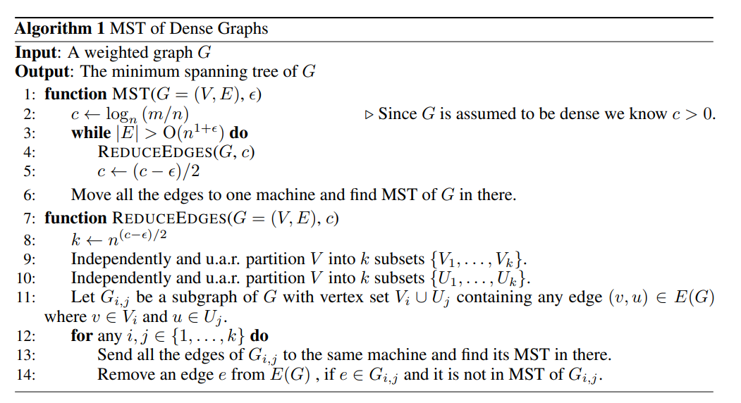 |
|---|
| Distributed MST Algorithm |
The algorithm is really quite simple. The main idea is that we can independently process each subgraph of comprising a random pair of vertex sets in a distributed fashion. Each worker finds the MST of the subgraph assigned to it, and any edge that is in but not in may be removed from the global edge set . In this way, we can whittle down the number of edges in until it is a small set that can fit in memory (i.e. in the order of which is not much larger than the number of nodes). Then we can just run MST one final time on the master node.
So the algorithm really hinges on Lemma 6 in the paper, which tells us that removing edges in this distributed way will still give us the correct MST at the end.
My proof by contradiction. Suppose an edge exists between nodes . Let denote a subgraph containing nodes , and suppose for contradiction that but .
First cut by removing the edge such that are in different partitions (each partition is a set of nodes). Observe that since exists in , it must be the lowest weight edge connecting and , since otherwise we could have replaced with a lower weight edge to complete the MST.
Now consider the subgraph and partition the nodes in according to to form and . Consider the MST of (might be a Minimum Spanning Forest instead, if not all nodes can be connected), and observe that there must exist a path between and in . Now remove any edges that cross and (call this edge set ). Then add back all the edges in that do not connect a path between nodes and .
Now there must exist exactly one edge remaining in that connects a path from to , since (i) a path exists between and in and (ii) there cannot be more than one edge that does so, otherwise there would have been a cycle in . We also know that this edge is not .
But is the minimum weight edge between and , and therefore it must also be the minimum weight edge between and . Hence this other edge could not have been in the MST of . We reach a contradiction.
Thus we are justified in removing edges in this way. This lemma is great because it allows us to independently process each subgraph, and if memory is of concern, we can also batch the number of subgraphs processed at each step according to the number of workers we have.
Lastly, note that is a dynamic parameter in the algorithm that measures the density (i.e. number of edges relative to number of nodes) of the graph at each step. Since we reduce the density of the graph in every step, is stepped down progressively. This also results in being stepped down progressively, where controls the number of subgraphs at each step. We start with a large , which requires less memory since small subgraphs implies that many edges are "chopped off". As the graph becomes less dense, we can afford to lower progressively and remove more edges.
Implementation
I can't seem to find an implementation of this algorithm, but it is probably easy to write a naive version of it using multiprocessing in python. We could store the edges in a sqlite database and distribute a batch of subgraphs at each turn, collect the edges to remove in the master and remove them from the db, and repeat.
Guo 2017 - DeepFM
Guo 2017 is an important innovation for recommender systems. The task tackled in this paper is to predict clickthrough rate (CTR) of recommended items.
The paper argues that it is important to learn implicit interaction signals between user and item features. Suppose we define the
- Recency of an item is an
order-1signal - Item category and timestamp is an
order-2signal, since e.g. demand for food items spikes at meal times - Gender, game category and user age is an
order-3signal, since e.g. male teenagers prefer shooting games
One can see that both low and high order signals are important for modelling CTR, and manual feature engineering is cumbersome to derive all such interaction rules. Hence we would like to have a deep learning model that can model such signals directly from raw user / item features and interaction data. This paper proposes to use Factorization Machines to model low order feature interactions and deep neural network to model high order feature interactions.
Setup
Suppose we have a dataset comprising n instances of tuples , where is an m-fields raw feature record where each field could be categorical or numerical. Each categorical field is represented as a vector of one-hot encoding, and each continuous field is represented as-is. Let denote the vector representation of field j (where dimension of numericals is 1 and dimension of categoricals is the number of categories), and denote the flattened vector of the laid out horizontally.
DeepFM
DeepFM comprises two distinct models: the FM component and the deep component which are simply summed together: . We go into each component below.
The FM component is a factorization machine that captures order-1 and order-2 interactions between the raw features. We first project each feature field to a k dimensional latent vector using a learned embedding matrix (in the paper, the authors set k=10). The latent vector representation of field j is denoted as . We compute the FM output as follows:
The first term represents the order-1 representation of the features as-is. The second term is a pairwise inner product between the embedding representations of each feature field, which represents order-2 interactions between the features.
The deep component tries to capture higher-order interactions between feature fields. This is done simply by laying out the embedding vectors horizontally, such that we form a flat input vector of size k \times m, and we call this . This fixed size vector is then fed into a multi-layer perceptron (or dense neural network) to finally return a sigmoid output. The standard forward equation for layer of the MLP is denoted below. Note that the embedding layer is shared between the deep and FM networks, allowing the deep component to benefit from the faster learning of the FM component.
In the paper, the MLP is of the form 400->400->400. Dropout is set to 0.5.
Implementation
Huawei has an implementation of DeepFM (amongst other models) in pytorch.
Van Den Oord 2017 - VQ-VAE
Neural Discrete Representation Learning
This paper proposes a Variational Auto Encoder (VAE) that uses discrete (categorical) latent variables instead of continuous ones. Discrete latents are more desirable from an interpretability perspective, but historically have not been able to perform as well as continuous ones. This paper is apparently the first to bridge this performance gap.
We are in the domain of computer vision, where the VAE is used to generate new images from existing ones.
Note that although VQ-VAE starts with the VAE framework, it is not strictly variational because of the deterministic operations within. It is more precise to call it a (deterministic) autoencoder with vector quantization regularization.
VAEs
A quick recap on regular VAEs:
- We start with some input which is an image
- The encoder encodes the input using into latent space
- Where in this paper is a discrete latent variable
- is the prior distribution (a uniform categorical in this paper)
- is the decoder that decodes a given latent back into input space (i.e. generates an image)
VQ-VAE
In VQ-VAE, the prior and posterior distributions are categorical. Drawing from the categorical distribution gives us an index which is used to index into an embedding table comprising dimensional embeddings. This extracted embedding is then used to represent the sample and fed into the decoder model.
More specifically, let us define a latent embedding space . That is, we have discrete latents and is the embedding dimension of each latent. Starting with an input , we pass it into the encoder to produce , which is a grid of -dimensional vectors. We then find the nearest embedding to in the embedding table to get a categorical index and a corresponding embedding for each encoded vector.
Note that using our running example of image generation, is encoded into a 2D grid of latents (say
32 x 32 x D). We find the nearest embedding at each position such that we end up with a grid of32 x 32codebook indices. Since each position is discretized independently of the others, in the exposition we refer to and so on as though it is one vector.
One way to think about this operation is that we are applying a particular non-linear operation that maps . Noticeably, this non linear operation is non-differentiable, which we will need to tackle later on.
We can thus define the posterior probability distribution for as:
Note that this posterior distribution is deterministic. If we define a simple uniform prior for , we get that the KL divergence is constant: .
Recall that:
Since if and otherwise, only one term in the summation is non-zero:
Hence the KL divergence term is constant and ignored during training.
Learning
At this point, we have fully specified the forward pass:
- Start with input
- Encode into
- Use embedding table lookup to find nearest neighbour
- Decode into
But it is not yet clear what the optimization objective and gradient flow should be. Recall that the standard VAE objective is to optimize:
The first term is the reconstruction loss, where we draw from the distribution that maps an input (using the encoder plus some random noise). Then we decode the back into input space and try to make it similar to input . The second term is the KL divergence which tries to regularize the distribution to be as simple as possible.
However, we cannot simply use this equation for the VQ-VAE:
- While the reconstruction loss is no issue (we can use the standard gaussian formulation), the second KL divergence term is a constant as we saw above. Hence doing this naively just reduces to a standard deterministic auto-encoder.
- Another problem is that in computing , we have to go through the non-linear operation of looking up the embedding table. This does not allow the gradient to flow back into the encoder.
Hence the authors need to re-design the optimization objective.
The first decision is to use the straight through estimator to circumvent the gradient issue. For the non-linear operation , we compute the forward pass normally (i.e. embedding table lookup) but simply pass the gradients through during backpropagation. This means that we approximate:
This allows the encoder to still receive gradient updates despite the non-differentiable operation. The theoretical justification for this operation is given in an earlier Bengio 2013 paper. Intuitively, if is close to , the gradients should still be meaningful.
The second decision is to use l2 distance to learn the embedding table. This is a form of dictionary learning. Specifically, we add a term to the loss:
Note that:
- here refers to the closest embedding to a given . We want embeddings in the codebook to move toward the average encoded representation
- is the stop gradient operation (e.g.
.detach()in pytorch). It uses the value of but does not pass gradients back to the encoder. Since the objective of this loss term is to learn the codebook, we do not wish to pass gradients back to the encoder
The third decision is to add a commitment loss to bound the encoder outputs. This part feels a bit more arbitrary. The authors say that with just the first two terms, there is nothing that tethers the encoder output, which can grow arbitrarily and perpetually be far away from the codebook embeddings. The solution is to include the reverse direction from the dictionary learning loss:
Notice that this is identical to the second term except that the stop gradient operator is applied to the codebook embedding. Thus this gradient pushes the encoder embedding to be closer to its nearest codebook embedding. is a hyperparameter but the authors observed that results were robust to a wide range of values (0.1to 2.0).
A natural question is to wonder why we need both the second and third term which are identical except for where the stop gradient is placed. Why can't we just do in a single term?
It appears that this will result in unstable training, because both sides (encoder and codebook embeddings) are simultaneously moving. This is a common issue in training things like GANs. Separating the terms results in more stable training.
There is also a close connection between VQ-VAE and k-means clustering (as a special case of expectation maximization). The step of assigning each encoder output to the nearest codebook embedding is akin to assign a cluster for each data point in k-means. The step of updating the codebook embedding is akin to updating the cluster centroids in k-means. This idea is explored in subsequent papers like Roy 2018.
Hence, the final training objective becomes:
Evaluation
The log likelihood of the complete model can be evaluated as the total probability over all latents . It is common practice to compute the log likelihood of a held out test set to evaluate how well our model has learned the data distribution:
Note that is also computed to report bits per dimension, which is a common way to evaluate such VAE models on test data. This is literally the number of bits required to represent our data under this model.
Because the decoder is trained with from MAP-inference, the decoder should end up placing all probability mass on after full convergence and no probability mass on . So we can write:
Learning the Prior Distribution
Up to this point, we assumed that the prior is a uniform categorical for training the encoder, decoder and codebook embeddings. This may be viewed as a training trick or mathematical convenience to make our framework work. As you may recall, using the uniform prior resulted in a constant term for the KL-divergence, meaning that the term is ignored during training.
At inference time, when generating a new image, using a uniform prior will result in incoherent images. Instead, we need to train a separate decoder like a pixelCNN or transformer over the latent space to generate a coherent latent grid for decoding.
Specifically, we encode and quantize our training dataset into grids of 32 x 32 codebook indices. Then, an autoregressive decoder is trained to predict the codebook indices in a causal autoregressive way. For PixelCNN, it works on the 2D grid of 32 x 32, but for transformer we need to linearize it in row-major form before training.
Now at inference time, we can start with a uniform latent index for the first position, then generate the subsequent positions using the latent decoder. After we have generated a grid of 32 x 32 latents, we look up embeddings to get 32 x 32 x D grid. This is passed to the decoder to get the generated image.
- Note that since we are doing autoregressive generation in the compressed latent space, it is a lot faster than autoregressive generation in the original pixel or token space. This is the idea used in Kaiser 2018 - Fast Decoding in Sequence Models using Discrete Latent Variables.
Hamilton 2017 - GraphSAGE
This paper presents a framework to efficiently generate node embeddings, especially for previously unseen nodes. It calls this inductive learning, i.e. the model is able to generalize to new nodes, as opposed to previous frameworks which are transductive and only learn embeddings for seen nodes. For example, matrix factorization methods are transductive because we can only make predictions on a graph with fixed nodes, and need to be retrained when new nodes are added.
GraphSAGE (i.e. Sample and Aggregation) aggregates feature information from the neighbourhood of a node to represent a given node. Feature information can include structural information (e.g. degree of a node) or other content-based information about a node, e.g. description of a job for a job node etc.
Setup
We start with a graph that is provided by data. We have input features . For a user-chosen depth of , we have aggregator functions and weight matrices . We also have a neighbourhood function , which means it maps from a node to a set of nodes in . Note that is the powerset of the set , i.e. the set of all possible subsets of . We wish to generate low-dimensional, dense vector representations of each node .
Forward Propagation
The algorithm for the forward propagation (in words) is as follows:
- We start with hidden representations , i.e. at layer 0, we just use the input features to represent each node
- At depth , we perform a neighbourhood aggregation step at each node :
- The aggregated vector is then passed through a dense layer to get the hidden representation at depth . Note that represents a non-linear activation, such as
ReLU: - We L2-normalize each vector
- We then repeat this process repeatedly for depths
- We then take the last layer:
The intuition behind the forward propagation is that we use the neighbours of to represent it. Importantly, we also include the hidden representation of the current node from the previous depth (analogous to a residual connection). At each depth level , we increasingly pull more information from further reaches of the graph. Note that in the aggregation step, a subset of each node's neighbours are sampled uniformly (as opposed to taking the full neighbour set) to control the complexity of the algorithm.
Loss
To train the weights, we define an unsupervised loss based on how well the embeddings are able to reconstruct the graph. Specifically, we have a loss which:
- Rewards positive pairs for having a high dot product
- Penalizes negative pairs ( being sampled negatives according to the negative sampling distribution )
Alternatively, we can also define a supervised loss based on classification cross entropy loss, with presumably some form of negative sampling. The authors did not elaborate on this.
Aggregation Methods
The authors explored a few ways to define the function to aggregate neighbour embeddings together:
GraphSAGE-mean: The element-wise mean of the neighbour embeddings is takenGraphSAGE-GCN: Same as above, except that the current node's hidden representation from the previous depth is not included. The experiments show that omitting this residual connection actually leads to significant performance degradation.GraphSAGE-LSTM: An LSTM is fitted over the sequence of embeddings. Since there is no inherent order to the neighbours, the authors randomize the ordering for each training sampleGraphSAGE-pool: An additional linear layer is added over the sequence of embeddings, before an element-wisemax-pooloperation is carried out
Generally from the experiments, it seems that GraphSAGE-mean is sufficient.
Ma 2018 - Entire Space Multi-Task Model
Ma 2018 tackles the problem of building a post-click Conversion Rate (CVR) prediction model. Note that CVR is the task of predicting conversions from impressions, whilst click-through rate prediction (CTR) is predicting clicks from impressions.
In a typical recommender system, users follow the sequential process of impression -> click -> conversion, where conversion may refer to making a job application, purchase action etc. Usually, CVR models are built the same way as CTR models: a dataset of clicked impressions is prepared, and the converted items are labelled as relevant. A model is trained on this dataset and then used to make conversion predictions on all impressions. This paper argues that there are two problems with this approach:
- Sample Selection Bias (SSB). The distribution of the training set (comprising only of clicked impressions) differs greatly from the distribution of the testing set (comprising all impressions), and this distribution shift will hurt generalization performance of the trained model.
- Data Sparsity (DS). The dataset for CVR (clicked impressions) is typically much less than the dataset for CTR (all impressions), and the lack of data makes model fitting difficult. The paper estimates that CVR dataset is typically
4%of that of CTR dataset.
Setup
Denote the observed dataset to be , with each sample tuple representing one impression drawn from a distribution with domain . is the feature space, and are label spaces (i.e. 0 or 1). Each feature vector captures all the user attributes, item attributes or user-item interaction for the impression event. The notation represents the sequential nature where a click event must precede a conversion event .
We can denote the various prediction tasks as follows:
- Post-view clickthrough:
- Post-click conversion:
- Post-view click + conversion:
The conventional way of modelling pCVR is to construct a sample from only click impressions, i.e. , where clicked but not converted impressions are treated as negative samples. We can see than . As mentioned above, there are problems with this approach.
ESMM Model
The ESMM model breaks down the pCTCVR task into its constituents, and uses two neural networks to model pCTR and pCVR simultaneously. Based on the diagram, it seems to embed each user field and item field into a fixed-size embedding, where the user field embeddings are summed up element-wise to produce an overall user embedding. The same is done to produce an overall item embedding. The user and item embeddings are then concatenated together, and this combined embedding is fed into a dense layer to finally output a real score representing either pCVR or pCTR. The two scores are then multiplied together to form the final prediction of pCTCVR.
Importantly, the projection (or lookup) layer from raw features to embedding is shared between the two neural networks. This allows the pCVR network in particular to benefit from the richer sample data that the pCTR network enjoys and addresses the data sparsity issue.
 |
|---|
| ESMM Model Architecture (Figure 2 from ESMM Paper) |
Finally, the model is trained with a multi-task objective. Specifically, the losses are computed on the dataset with all impressions. The output pCTR is compared against clicks using a cross-entropy loss, and the output pCTCVR is compared against conversions using a cross-entropy loss. This multi-task loss allows us to exploit the sequential nature of the data generation process, such that only needs to model the delta aspect that leads from a click to a conversion.
The authors show that modelling in this multi-task manner outperforms a setup where two models are trained independently to predict CTR and CVR respectively, and their product is taken to estimate pCTCVR. Unfortunately, we cannot replicate this joint-task learning setup with gradient tree-based models, at least not naively.
Details
The authors set the dimension of each embedding vector to be 18, and each MLP is 360 -> 200 -> 80 -> 2 dimensional. Adam solver is used with .
Kang 2018 - SASRec
Self-Attentive Sequential Recommendation
This paper uses a transformer model with self causal attention to perform recommendations, by representing each user as a sequence of item embeddings and predicting the item interacted at time t+1 by using all the information up to time t.
Background
This paper came out shortly after the transformer (Attention is all you need) was invented. Up to this point, sequential recommendation was performed using Markov Chain methods or RNN-based methods. Since the self-attention mechanism of transformers is well suited to sequential modelling, this paper makes the natural adaptation of self-attention to the recommendation task.
Setup
In the setting of sequential recommendation, we have for each user a sequence of item interactions where each element represents an item. For computation reasons we may choose to truncate to the most recent interactions. For simplicity we may also denote . We have user and item sets . Let us also define:
- as the full item embedding matrix with latent dimension
- as the learned position embedding matrix
For each user, we receive and truncate it to the most recent items. If there are less items, we left-pad the sequence with a constant zero vector. This results in an input embedding matrix for the user.
Analogous to the language modelling task, the targets for each user is simply shifted to the left by one. In other words, the target at time step would be the item interacted with at time step .
Model
Position Embeddings. We start by adding position embeddings to the user representation; absolute position embeddings are used here. Since this is a transformer model, the model has no notion of the item sequences if we do not inject the position embedding, and would not be able to learn that more recent items contain more valuable information about the next item to predict. The authors later show that visualizing the self-attention heatmap reveals that without position embedding, all items are attended to similarly, but with position embedding the attention weights are concentrated near the diagonal, i.e. more recent items are attended to stronger.
Specifically, we simply add the position embedding matrix to the input embedding matrix, such that:
Self attention. The standard scaled dot product attention is used to perform self attention on the input embedding. Specifically:
Where are the projection matrices. We then make sure to mask the softmax attention matrix in a causal manner, so that there can be no interaction between and for all .
Feedforward network. A point-wise two-layer feedforward network is applied to the output of the self attention (i.e. ), like so:
Where and . Note that in the feedforward networks, there remains no interaction between any at different time positions.
Stacking self attention layers. Now we stack the self attention layers and also apply (i) residual connection, (ii) dropout and (iii) LayerNorm each time. This is standard practice in transformers and leads to more stable training.
Where we define the composite function as follows, and is defined similarly.
Note: In modern transformers, the is replaced by the simpler and the function is replaced by the function.
This gives us the full specification for one layer (layer ) of the transformer. Several layers are stacked to provide the full model.
Prediction. After the final layer, we have as our representation. The predicted score at each time step for any item is made according to a simple dot product:
Training Loss
As discussed above, the target for each time step is simply the next item at time step . Specifically, if we define as the target output at time step , we have:
- if is a padding item
- for
Note: Not sure if we need to predict the padding item, or just simply mask the loss at those positions. Similarly for time step , where we do not know the next item to predict after the last item in the sequence.
Finally, the binary cross entropy loss is chosen as the objective function for each time step . Specifically, a random negative item that user has not interacted with is sampled for each time step and used as the negative example. The loss is:
Note: The binary cross entropy loss is chosen here with one sampled negative per time step. A later paper Turning Dross Into Gold Loss: is BERT4Rec really better than SASRec? will show that using softmax cross entropy loss with many sampled negatives will lead to much better performance.
Experiments
For the experiments, two attention layers were used (i.e. ). Item embeddings are shared between the input embedding layer and also used in the prediction layer (for ). The latent dimension is set to .
The ablation studies found that:
- Increasing number of layers saturates at around
- Using multi-head attention did not improve over single head attention
- The absolute position embeddings generally improved performance relative to no position embeddings
Implementation
The authors endorsed a pytorch implementation here.
Kaiser 2018 - Fast Decoding in Latent Space
Fast Decoding in Sequence Models using Discrete Latent Variables
This paper uses the idea in VQ-VAE to do fast decoding in latent space.
Main Idea
Transformers parallelize during training well, but are slow at inference due to autoregressive nature. This paper proposes to autoregressively generate in discrete latent space instead, which can be much faster depending on the compression:
- First auto-encode target sequence into discrete latent space which is a shorter sequence
- Train a decoder to generate in discrete latent space autoregressively
- Decode output sequence from the shorter latent sequence in parallel
Here is an infographic from nano banana that captures the idea of generation in latent space:
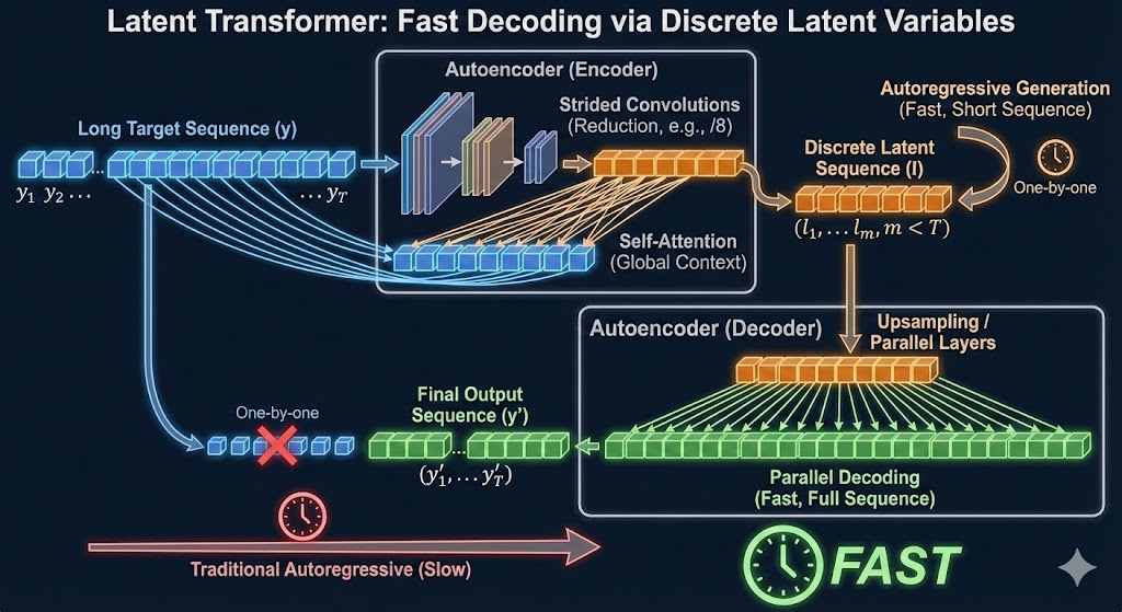 |
| Fast Generation in Latent Space |
Setup
When generating sequential output, autoregressive models generates in a canonical order. This is because the model is trained to predict:
During training, because ground truth is known, we can train in parallel. During decoding, this is a fundamental limitation.
The proposal is to first encode the original sequence into a shorter sequence of discrete tokens , where is much smaller than . This latent sequence is also autoregressively predicted, and subsequently decoded in parallel back into the original token space. In the experiments, .
Latent Transformer
The latent transformer is described in terms of a machine translation task. Given an input sequence in English, and a corresponding output sequence in German, our input-output pair is .
The high level architecture is:
- The function will autoencode into a shorter sequence of discrete latent tokens using some discretization technique
- The latent prediction model which is a transformer will autoregressively predict based on
- The decoder is a parallel model that will decode from and the input sequence
Loss
The reconstruction loss compares the encoded - decoded output to the original target sequence :
The latent prediction loss compares the true latents generated by the autoencoder to the generated latents :
The final loss is the sum of the two:
Autoencoder
Now we describe each part in more detail. The diagram below summarizes the architecture of the autoencoder .
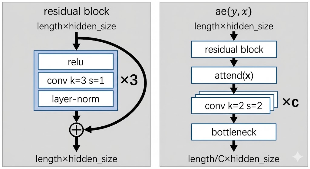 |
| Autoencoder architecture |
The input to the autoencoder is of shape length x hidden_size. The aim is to shorten the sequence length by downsampling using convolutions.
We first pass through a residual block which aims to learn local features using convolutions:
- Pass through
relu - Pass through 1D convolution with
k=3, s=1. This means we look over a window of3tokens each time, and take a step of1token each step.- Since stride is
1, the sequence length is unchanged
- Since stride is
- Pass through layer norm + add the residual connection
Then we pass through a standard self attention block.
Then we pass c times through a downsampling convolution:
k=2means that we look over a window of2tokenss=2means that we stride over2steps at a time: this effectively halves the sequene length- Doing this
ctimes means we get reduction in length
Finally we pass through the bottleneck function, which has yet to be described. But essentially the bottleneck function converts the representation of hidden_size at each position into a discrete token, and then represents it instead by the embedding of the discrete token using a lookup.
Decoder
The decoder decodes from latent space back into token space.
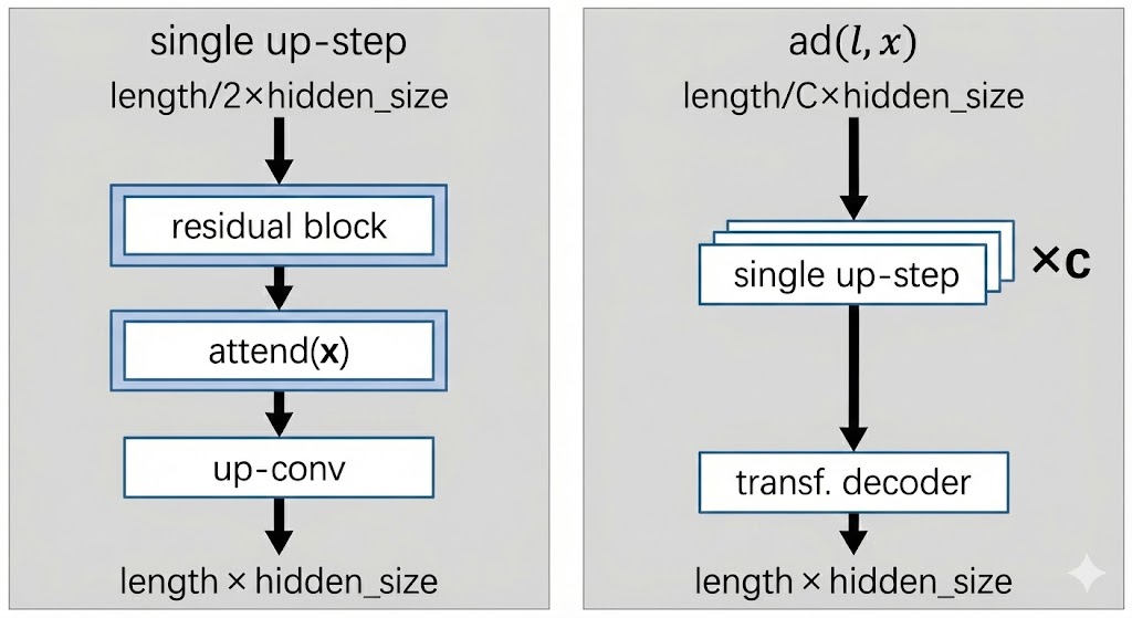 |
| Decoder architecture |
We first pass through c up-steps, each of which will double the sequence length of the encoded sequence:
- The same residual block from before is used
- Self attention layer is used
- An up-conv step is performed:
- A standard feed forward MLP is used that doubles the hidden dimension
- A reshape operation is done to translate the extra hidden dimension into sequence length instead
Finally, the decompressed sequence of length x hidden_size is fed into a standard transformer decoder to decode the target sequence .
- Note that for the first 10k steps of training, instead of feeding the decompressed sequence, the authors pretrain this decoder transformer model by feeding the target sequence (i.e. training it like a standard transformer decoder). This is to warm up the head so that gradients to upstream components are reasonable.
Discretization Bottleneck
This is actually the main part of the paper - how do we discretize our token sequence into latent space so that we can predict the latent tokens in an autoregressive manner?
The bottleneck function takes a target token embedding and maps it to a discrete token in :
- First, take and encode it: , where is the dimension of the latent space.
- Next, pass the encoding through a bottleneck to product a discrete latent token
- Look up embedding table using to produce an embedding to pass to the decoder
Note that the bottleneck function is applied to each sequence position in parallel, indepedently.
Gumbel Softmax
The gumbel-softmax trick is found in Jang 2016. It is a popular discretization technique.
First, we project the encoder output using a learned projection matrix , such that we get logits :
We can simply extract the discrete code for the decoder as:
For evaluation and inference, we can simply use to look up an embedding table to get . However, we cannot use this approach for training as the argmax and embedding lookup are non-differentiable.
For training, the Gumbel-softmax trick is used to make the whole thing differentiable.
- First, we draw i.i.d samples from the standard Gumbel distribution
- Then we compute the weight vector using a softmax, where for each latent dimension :
- Now we simply compute the input to the decoder as the weighted sum of the embedding table:
For low temperatures of , would be close to representing the 1-hot arg-max index of , which is what we use for evaluation and inference. Setting too high would cause divergence between training and inference, which is not ideal.
Why do we add the gumbel ? Ideally during training, we want the encoder logits to represent probabilities of a categorical distribution, from which we sample the discrete code . This ensures that we have:
- Exploration from the stochasticity
- Discretization. We also force the embedding to be a single embedding (i.e. discretization) rather than a smooshed average of several embeddings.
The gumbel-max trick tells us that choosing results in an index distributed exactly according to as dictated by the softmax of the logits, which is what we want.
Since the gumbel-max is not differentiable, we simply relax it into a softmax operation, giving us the gumbel-softmax.
Vector Quantization
The VQ-VAE is covered in VQ-VAE. Here is a brief recap.
- The encoder output is used to do nearest neighbour lookup on embedding vectors to give us:
- and
- Where
- The loss is the reconstruction loss + the commitment loss between encoder output and codebook vectors:
It turns out that the gradient update can be replaced by an exponential moving average over:
- The codebook embeddings ; and
- The count measuring the number of times is selected as a nearest neighbour
For a given mini-batch of target embeddings , we can update the exponential moving average for counts like so:
And the codebook embeddings updated as the average encoder output selected for :
is a decay parameter and set to in the experiments
Note. The paper also covers two other discretization techniques, namely improved semantic hashing and decomposed vector quantization (to counteract codebook collapse), but I don't cover it for now.
Results
The results show that the discretization bottleneck is not as good as a standard transformer, but beats all previous discrete methods and runs faster than a normal transformer.
Ablation results show that:
- Increasing the codebook size improves performance
- Increasing the ratio (i.e. shortening the sequence more aggressively) leads to speedup in inference but also clearly hurts performance
Hence it seems like there is no free lunch here.
Reimers 2019 - Sentence-BERT
Sentence-BERT (or SBERT) was one of the first papers to suggest a way to fine-tune BERT models to generate useful embeddings that can be used for search / retrieval.
Prior to SBERT, BERT models were mainly used for sentence pair regression tasks by passing two sentences into the transformer network and adding a classification head on top to produce a float value. We can call this the cross-encoder approach. In other words, researchers only cared about the final prediction and did not make use of the embeddings, or the final vector representation of the inputs. This approach is suitable for reranking a small number of documents but not for nearest neighbour search in a corpus with millions of documents.
Naively, one can element-wise average the BERT embeddings at the final layer to produce a vector representation of the text. This vector representation can then be used for nearest neighbour search or clustering. However, because BERT was not explicitly trained for this objective, it results in rather bad sentence embeddings, often worse than GloVe embeddings.
Method
The SBERT paper presents 3 different training objectives, all of which perform well on embedding similarity tasks. The choice of objective depends on the dataset:
-
Classification objective. This is for tasks where the objective is to predict a label given two sentences A, B. We pass each sentence into the BERT network and a pooling layer to get two vector representations, and . The pooling layer can be (i) take the
[CLS]token embedding, (ii) take the element-wise mean or (iii) take the element-wise max. We then create a concatenated vector which is fed into a softmax classifer. The network is trained using cross-entropy loss.Note that this siamese approach (where each sentence is passed into the same network) differs a little from the typical cross-encoder approach, where the sentences are concatenated as a string with the
[SEP]token before passed into the network. The latter approach is presumably more powerful because the attention mechanism can attend to all pairwise relationships -
Regression objective. This is for tasks where the objective is to predict a float given two sentences A, B. Given the vectors and , the cosine similarity is simply taken to generate a float between and . The cosine similarity is then compared with the actual float value using mean-squared error to generate a loss.
-
Triplet objective. This is for tasks where each data point is a triplet (anchor sentence , positive sentence , negative sentence ). We then minimize the loss function, where is the margin:
Ablation
- Pooling strategy. Using
[CLS]or mean seems to be largely similar. The authors saw some degradation using max for the regression objective. - Concatenation. For the classification objective, the concatenation strategy makes some difference. In particular, using yields but yields . Thus the element-wise difference is important in yielding useful embeddings, probably because it can be used to push similar sentences together and dissimilar sentences apart. The authors also found that adding element-wise multiplication does not help.
Takeaway
It is interesting that the classification objective, which is close to a cross-encoder framework, is also able to learn useful embeddings by adding the difference operation . This suggests that we can train a cross encoder and simultaneously get useful embeddings for nearest neighbour retrieval at the same time.
Yi 2019 - LogQ Correction for In Batch Sampling
Yi 2019 - Sampling Bias Corrected Neural Modelling for Large Corpus Item Recommendations
This paper proposes a way to perform logQ correction for sampling bias introduced by in-batch negative sampling when training two tower models. The algorithm proposed is a streaming algorithm that estimates item frequencies based updates after seeing each mini batch.
Setup
Let , denote a user and item respectively, where there are users and items. Let and denote user and item embedding functions that map each and to . These functions are typically:
- Some sentence transformer model for texts
- Some hash embedding in the collaborative filtering setting
The output of the model is the inner product of the embeddings, i.e. . The goal is to train the model from a training dataset of user-item interactions, denoted by , where , are the interacting query and item and is the associated reward.
- Typically to denote an interaction
- We can also use to denote some quality weight, e.g. time spent on product
Given a query , we typically model the conditional probability of picking item based on the softmax function. parametrizes the embedding model:
We then design the loss function as a weighted log likelihood of the training interactions:
In Batch Sampling
In practice, the denominator for above is not feasible to compute when the number of items is very large. The common practice is to sample only a subset of items that are drawn in a mini batch. Hence given a mini batch of B pairs and for any , the batch softmax becomes:
Note that each refers to a positive pair. However, the batch softmax above is usually a very biased estimate of the full softmax. This is because our training data usually has a heavy bias toward popular items, hence the likelihood of a popular item being included in the denominator is usually quite skewed.
In other words, our model trained with this biased likelihood function may have a low training loss against popular items in the denominator during training. But when used in retrieval, the model may be assigning high scores to rare items that should be negatives, just that our model did not have a chance to discriminate against them due to the biased sampling during training.
This issues underlies the common phenomenon when training such retrieval embedding models where the reranking performance is good but retrieval performance is very bad. The reason is that reranking is often performed against popular items that the model sees often, but retrieval by definition searches across the whole item catalogue. Hence retrieval is (from this perspective) a harder task than reranking. Special attention must be paid during training to ensure that the model learns to discriminate well against all items in the catalogue, and this logQ correction is one of the methods at our disposal.
In Adaptive Importance Sampling to Accelerate Training of A Neural Probabilistic Language Model, the authors propose the following way to correct the biased batch softmax by correcting each score logit:
Where denotes the probability of sampling an item in a random batch. With this correction, we can denote the batch softmax as:
And finally we have the batch loss function as:
Estimating Sampling Probability in Stream Setting
Notably, the batch loss function does not require holding a fixed set of items in memory to serve as negative candidates, making it suitable for use in a streaming training data setting. Thus, the authors propose a method to estimate the sampling probability in a streaming fashion as well.
The first observation is that it is easier to track the number of steps (or batches) between two consecutive hits of item . e.g. if we only get one item once every 50 batches, then . The proposed algorithm is as follows:
- Initialize Arrays with size
- Let be a hash function from an item ID to
- At batch , sample a batch of items. For each item in the batch:
- At inference time, the sampling probability for item will be .
Other Notes
The authors note that adding l2-normalization to embeddings improves model trainability and leads to better retrieval quality. Also, adding a temperature to each logit helps to sharpen the predictions. In their experiment, the best is usually around 0.05 (i.e. logits get multipled by 20x).
Zhao 2019 - Recommending What to Watch Next
Recommending What Video to Watch Next: A Multitask Ranking System
This paper covers Youtube's recommendation system for what video to watch next, given the current video. The main contributions of this paper are:
- Handling position bias
- Multi-gated Mixture of Experts to handle multi-task objectives
Background
This paper focuses on the ranking task of next video recommendation. There are specific challenges to their setting:
- Multiple signals. For each video recommendation, there are engagement signals such as clicked, duration watched etc., and also user satisfaction signals such as liked, shared etc. Optimizing for these tasks is potentially conflicting, but multi-task learning also has potential to learned shared representations across tasks.
- Position bias. Position bias can degrade recommender performance since it may learn signals irrelevant to relevance. Tackling this issue can lead to online performance gains.
- Large Scale. The industry scale of recommending from billions of videos means that training quality might need to be traded off for efficiency. For this reason, the paper opts for a neural network based point-wise ranking model (as opposed to pair-wise or list-wise training methods like InfoNCE). This is also why the paper focuses on an architecture that can efficiently share parameters between different input feature modalities and prediction tasks.
The candidate generation is performed using multiple retrieval models, each of which captures a different aspect. For example, one algorithm matches topics of the query video, whilst another is based on co-watch statistics. A sequence model similar to Covington 2016 - Deep Neural Networks for YouTube Recommendations is also used. The efficient gramian methods in Krichene 2018 - Efficient Training on Very Large Corpora via Gramian Estimation was also used.
For ranking, a few hundred candidates are retrieved and passed to the ranker. Point-wise ranking loss is chosen for simplicity and scaleability.
Mixture of Experts
It is common for ranking systems to have multiple objectives, due to having multiple implicit feedback signals in a recommender system. There are some approaches to deal with this:
- Explicitly modelling the relationship between the signals. E.g. in ESMM, the conversion probability head is modelled as a multiplication of the click probability with a separate head. In this way, the conversion head only needs to learn the "delta" signals that cause a click to turn into a conversion. However, such an approach only works when the relationship between tasks is known, and is also not very scaleable when the number of tasks increases.
- Shared Bottom Layer. The typical architecture is to have a shared representation layer at the bottom (from the inputs), and then to have a task specific head for each task connected to this shared bottom (see figure below). However, such hard parameter sharing has been shown to sometimes harm the learning when correlation between tasks is low.
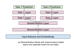 |
|---|
| Shared Bottom Architecture |
The mixture of experts architecture proposed is covered in Ma 2018 - Modeling Task Relationships in Multi-task Learning with Multi-gate Mixture of Experts. The main idea is that we have several expert layers that branch off from the shared bottom, and we also have a gating head (ending in a softmax) for each expert tower. The representation for each task is thus a unique weighted combination (the weights coming from the gating heads) of the expert layers. This somehow allows the model to "distribute work" to different experts to modularize information for each task. Note that the number of experts can differ from the number of tasks.
Specifically, focusing on task , let us denote:
- as the representation arising from the shared bottom layer
- as the expert where .
- In this paper, is simply a sequence of ReLU layers.
- Here I denote the expert representation as having the same dimension for simplicity but that does not need to be the case.
- is the gating weight for task from the expert
- is the vector form comprising elements for experts
- It is obtained by
- Where is the gating weights for task
- is a final sequence of ReLU layers for task
Starting from the shared bottom representation , for each task we perform:
- Obtain the gating weight vector
- Obtain the weighted representation for task as
- Obtain the final prediction logit for task as
We see that this architecture is quite flexible in supporting an arbitrary number of experts and tasks. In contrast to ESMM, we do not need any knowledge of how the specific tasks relate to each other to specify this network.
The authors mention that in distributed training, there is a danger that the softmax gating network may experience an imbalanced expert distribution problem, where gating networks converge to have zero-utilization on most experts. They experienced this 20% of the time. To mitigate this issue, dropout is performed on the gating networks by setting the softmax weight for each gate to be 0 with probability 10%. The softmax vector is then renormalized to sum to 1 after the dropout. With this approach, they completely eliminated the polarization issue. It is not clear whether this issue happens in single-machine training, but nonetheless the fix seems easy to implement and seems like a low-hanging fruit to do.
Position Bias
A common problem with implicit feedback data is position bias, i.e. the propensity of users to click items in higher positions due to the position rather than the relevance of the item. There are some ways to deal with this:
- Inject the position as an input feature in model training to learn the position bias, and then set this feature to a fixed constant when serving
- Learn the position bias explicitly from offline data or random experiments, then use methods like Inverse Propensity Scoring to regularize or normalize the predictions
The problem with the latter approach is that position bias is dynamic in real world systems, making it cumbersome to separately estimate it. Hence this paper adopts the former approach that is efficient and adapts to training data distribution changes as we train the main model.
This paper treats position bias as a bias term that is added to the prediction logit for each task , before the logit is fed into a final sigmoid to generate a click probability. The position bias term is generated by passing the position feature and other features like device info into a shallow tower. Device info is included because different position bias is observed on different types of devices.
Note: The paper is not clear on how the position and device are represented as features. Naively, I imagine that a small embedding (say of dim 32) is used to encode each position and each device value. Since the position bias is strongest at the top positions, we could cap the number of position embeddings to say 50, and assign all later positions to the final position embedding. Then, we can concatenate the position and device embedding to form an embedding of say dim 64, and feed that into a shallow ReLU layer to generate the position bias logit. Another way is to do element-wise multiplication of the position and device embedding.
Training
The paper does not provide much detail on how exactly training is performed, but they mentioned that point-wise loss was chosen for simplicity. I would imagine the process to be something like:
- Start with positive training examples where some subset of engagement or satisfaction metric were observed (e.g. user watched)
- For each positive training example, sample one or more random negative(s) from items that were shown to the user in that context but user did not click
- Train the model to predict the multi-task outcome for each of these examples in a point-wise manner
Experiments
Online experiments were performed on YouTube. AUC was chosen for classification tasks and squared error for regression tasks.
- The paper found that using the shallow tower for position bias increases AUC by
0.24% - The Mixture of Experts approach is better than the shared bottom approach for the same number of model parameters.
Takeaways
This paper is scant on details on the actual ranker and features used, but makes a good case for the two proposed components of (i) mixture of experts and (ii) shallow tower for position bias.
Lee 2020 - Large Scale Video Representation Learning
Large Scale Video Representation Learning via Relational Graph Clustering
This paper proposes an efficient method to learn video representations from relational graph data (i.e. user item interactions). Specifically, it learns a small-ish embedding model that transforms raw audio-visual features for a given video into a vector representation that is useful for downstream recommendation tasks. This method seems to be in use at YouTube at least until 2023 as it was mentioned in Singh 2023 - Better Generalization with Semantic IDs.
This paper is in the genre of metric learning of similarity metric between videos. Similar to FaceNet, it uses triplet contrastive loss to push related videos together and random videos apart. The contribution of the paper is a hierarchical clustering approach to sample smart negatives which they show to be much more informative for learning than random negatives.
Setup
We start with a raw input representation of a given video , where could be a concatenation of various raw input features or a representation from some off-the-shelf pretrained embedding model. We are also given a relational graph where each node is a video and each edge represents some relationship between two videos. The edge weight can be binary or real numbers. We may obtain such edge relationships from implicit feedback, e.g. how frequently two videos are co-watched, co-clicked, co-searched, etc. The aim is to learn a representation where is much smaller than , such that if they are related and otherwise.
Method
The relational graph is pre-processed with a hierarchical clustering algorithm. A hierarchical algorithm is chosen so that we can sample negatives with varying levels of difficulty later on. The paper uses Affinity Clustering, although it notes that any suitable clustering algorithm works as well. At a high level, affinity clustering at each step chooses the lowest outgoing edge-weight to add from each cluster. Some desirable properties of affinity clustering are (i) tends to produce clusters of similar size, which helps negative sampling to be consistent across clusters and (ii) easily parallelizable.
Once we have the relational graph and clustering , the training proceeds as follows:
- Construct triplets:
- Sample a random
anchorvideo from all videos - Choose a
positivevideo from its neighbours in - Sample a
negativevideo at a desired level from sibling clusters in
- Sample a random
- Compute the distances for each triplet :
- Anchor-positive distance:
- Anchor-negative distance:
- Perform online semi-hard negative mining:
- In each mini-batch, resample negatives to choose the hardest semi-hard negative in the mini-batch for each row
- Recall that a semi-hard negative is where
- So we are choosing negatives such that is as close as possible to without being lower
- Note that this means we need to compute for all anchor-negative pairs in the mini-batch
- Optimize for the following objective:
This is essentially the same procedure as FaceNET, except the smart and dynamic choice of negatives. Also note that since we only train with semi-hard negatives, the inner term , so the operator on the loss can actually be ignored.
Denote the anchor video as A. The smart negative sampling from sibling clusters is defined as:
- At
L0, negatives are chosen from all the descendants of from the affinity tree - At
L1, negatives are chosen from all the descendants of - And so on
Experiments
The embedding network is simply a fully connected MLP with layers of dimension 4,000 and 256 respectively. Each video is preprocessed into an embedding representing raw audio-visual features using techniques like fourier transform, feeding into pre-trained audio-visual ResNets etc. and fed into the MLP to get a resulting embedding.
The relational graph is constructed by adding an edge between a pair of videos if they are frequently co-watched by multiple users. Specifics are not provided but I presume the rule is something like co-watched by at least n user pairs. In other words, the edge rule sounds fairly stringent to minimize the number of false edges. The videos are then split into training and test with a 7:3 split. Each mini-batch comprises 9,600 triplets and the margin is set to 0.5. The learning rate starts at 0.1 and decays by 0.98 for every 300k steps.
The evaluation simulates a cold start scenario, where both the query video and candidate videos are all taken from the unseen test set. For each query video, retrieval is performed using the model (using cosine similarity) on all videos from the test set. The NDCG and MAP are then computed based on whether we successfully retrieved relevant videos for the query video based on the true relational graph .
Findings:
- Smart negatives are significantly better than random negatives. To further prove this point, the authors tracked the % of negatives that remain the same after the hard negative re-sampling step, and showed that a much larger % of smart negatives were retained (10% to 15%) than random negatives (close to 1 /
batch_size). Interestingly, the usage % of smart negatives actually increases steadily as training goes on. This could be because at the start, many smart negatives are too difficult for the model and do not qualify as semi-hard. As the model learns, it is able to handle more smart negatives and the usage % increases. - Online semi-hard negative mining is important. The authors found that using smart negatives without the online mining step does not perform well. This could be because the smart negatives are too difficult for the model at the beginning and the model fails to learn. The authors suggest that an alternative to the online mining step is curriculum learning, where easier negatives are provided at the start and difficulty is increased gradually.
- More difficult negatives work better. The authors tried training at
L0,L1andL2difficulty levels respectively, and found that training atL0consistently does the best. This kind of defeats the point of the hierarchical clustering, but I suppose it depends on the use case and in other settings other difficulty levels may work better.
Takeaways
This paper proposes a scaleable and easy-to-understand method of item representation learning. Obviously, it can be extended to other modalities such as text so long as we find a reasonable way to represent the raw inputs. For text, we can probably directly fine-tune some BERT encoder using the same procedure.
Nevertheless, note that this paper alone would not provide optimal performance if we use the embeddings here directly for retrieval. One big reason is that we are considering an undirected relational graph, so we learn only symmetric relationships, whereas in retrieval item sequence often matters. For example, people often progress from beginner videos to more advanced videos for a particular subject, and this paper would not be able to capture such relationships. Hence the embeddings in this paper have to be fed into another retrieval or ranking model for optimal performance.
He 2020 - LightGCN
He 2020 - LightGCN is a simple and effective Graph Convolution Network for recommendation.
LightGCN is an adaptation of Graph Convolutional Neural Networks (GCN) to the task of recommendations. In a typical Convolutional Neural Network for vision, convolution aggregations (such as linear projections, pooling, average) are applied to a neighbourhood of pixels that are near to one another. The aggregations transform the raw pixel values into a hidden layer of "embedding" values, and the next layer of aggregations is applied to the hidden layer, allowing the CNN to learn more abstract features with each increasing layer. A GCN uses essentially the same idea, except that the definition of neighbourhood of a node A are the neighbouring nodes that are connected by an edge to A. The GCN thus allows us to train node embeddings on all types of graphical data, such as social networks, user-item interactions etc.
Setting
This paper tackles the task of collaborative filtering without features, i.e. making recommendations purely from the user and item id. Also, no negative samples are required - all we need is edges between users and items based on some form of implicit interaction.
Neural Graph Collaborative Filtering (NGCF)
The LightGCN model is essentially a simplification of the NGCF model, so the paper starts here. Btw, there are some overlaps between LightGCN authors and NGCF authors. The setup is as follows:
- Each user and item are embedded from their
id->embedding - Let denote the ID embedding of user and denote the ID embedding of item
NGCF uses the user-item interaction graph (derived from data) to propagate the embeddings as follows:
Some notes about the propagation equations above:
- and denote the embedding of user and item respectively after
klayers of propagation - is a non-linear activation function
- denotes the set of items that interacted with user . For instance, it could be all the items the user purchased within the past 3 months. is the set of users defined in a similar way.
- and are trainable weights
Intuitively for a given user, the equation propagates (i) the user embeddings itself (order-1), (ii) the embeddings of neighbouring items (order-1) and (iii) the hadamard interaction between the user and the neighbouring items (order-2). And likewise for the item embeddings. Note that
Finally, after training the network of layers, we obtain embeddings for each user and item. The embeddings are concatenated as such and where are vectors of dimension . Prediction scores for the match between user and item are then computed via the inner product .
Problem With NGCF
The authors argue that NGCF is unnecessarily complicated because traditionally, the base embedding layer is derived from rich semantic features such as embedding the title of papers etc. This justifies the usage of the activation function and the projection weights etc. to learn a transformation of the semantic features. In contrast, for the collaborative filtering setting, the embeddings are arbitrary numbers tied to each user or item ID. Hence, performing multiple non-linear transformations will not lead to better feature learning.
LightGCN Forward Propagation
In LightGCN, we essentially remove the non-linear activation and weight projections. The propagation equations simplify to the following:
The final representation of each node (whether user or item) is then a weighted sum of its hidden representation across all layers:
Although could be a parameter to be optimized, the authors propose just setting for simplicity.
Noticeably, the forward propagation does not include the self-connection from the previous layer, i.e. the update for does not explicitly include , which other papers like GraphSAGE argue is important. The authors argue that because they use a weighted sum of hidden representations across all layers, this essentially is equivalent to including self-connections, so that is no longer necessary.
Loss
The only trainable parameters of the model are the embeddings at the 0th layer, i.e. . The authors propose using Bayesian Personalized Ranking loss, which is a pairwise loss that encourages the score of a neighbour to be higher than the score of an unobserved, randomly sampled counterpart.
In contrast to NGCF and other GCN approaches, the authors do not use dropout as a regularizer. Instead, they think the L2 regularization on the embedding layer is sufficient, as these are the only parameters in the model. Training of the model is done in a mini-batch manner, where batches of (user, item) tuples are drawn, negative items sampled, and the loss evaluated.
Ablation Studies
The paper has a few ablation findings:
- Symmetric Normalization is important, i.e. it is important in the forward propagation to divide by . Omitting either one leads to performance degradation. Note that in GraphSAGE, the
GraphSAGE-meanvariant essentially does , i.e. it only normalizes by the user degree. I suppose normalizing by the item degree as well penalizes popular items, so it could be useful. - Layer combination is important for robustness as we increase the number of layers, i.e. instead of just taking as the final embeddings, it is useful to take the element-wise mean of the embeddings at each layer. This might be analogous to the impact of including self connections.
Cornac Implementation
Cornac has a torch implementation of LightGCN:
The code relies on the dmlc/dgl package for constructing the bipartite user-item graph which will be used to compute neighbourhoods. The construct_graph function works as follows:
user_indicesanditem_indicesare lists of the same length where each element at indexicontains a pair of user, item that interacted- A
dgl.heterographis constructed with both directions:("user", "user_item", "item")represents user -> item direction("item", "item_user", "user")represents item -> user direction- Hence there are two node types and two edge types in the graph
- Starting with the
user->itemdirection:srcanddstare torch tensors containing the users and items respectively that interacted, both of lengthMdst_degreeis a torch float tensor of lengthMcontaining the number of users interacting with each item indstsrc_degreeis a torch float tensor of lengthMcontaining the number of items interacting with each user insrc
At model initialization, self.feature_dict is initialized with xavier initialization as follows. Note that because we have a heterograph, the nodes are defined as a dictionary of the form node_type: feature_tensor.
self.feature_dict = {
"user": user_embed, # (n_users, embed_dim)
"item": item_embed, # (n_items, embed_dim)
}
The GCNLayer class represents one layer of the message passing network.
References
Lewis 2020 - Retrieval Augmented Generation
Lewis 2020 - Retrieval-Augmented Generation for Knowledge-Intensive NLP Tasks
This paper proposes a way to fine-tune a parametric seq2seq transformers (e.g. GPT) with a non-parametric memory through dense retrieval. The main idea is to extend parametric memory (i.e. the "knowledge" that is stored within the LLM floating point parameters) of the seq2seq model by coupling it with retrieval of documents from a vector database (dubbed non-parametric memory, using Wikipedia articles in the original paper). We can update the non-parametric database's knowledge as the world changes.
The paper argues that this setup is ideal for knowledge-intensive tasks such as open question answering, fact verification etc., where it is impossible to store all knowledge in parametric memory.
Setup
Given an input sequence of tokens , we wish to retrieve contextual documents and use them as additional context when generating target sequence . We have two models:
- Retriever which returns top-k truncated probability distributions over text passages. Truncated probably means that the probability is normalized such that the top-k probabilities sum up to
1for each retrieval. - Generator parametrized by which generates tokens in an auto-regressive manner.
The goal is to train both models end-to-end on a fine-tuning corpus of input sequence / output sequence pairs. The loss objective is to minimize the negative log-likelihood .
Training
The paper proposes two different models to achieve the end-to-end prediction.
- RAG-Sequence. In this setting, we retrieve
kdocuments and keep using them to generate the entire target sequence.
- Note that we are marginalizing (or taking a weighted combination) over the truncated distribution of , implying that we trust each document according to its retrieval probability in the final probability for generating each token.
- The expression just means that we generate the target sequence with an input sequence that is a concatenation of , and .
- The retrieval is done using a BERT encoder using Maximum Inner Product Search (MIPS). To avoid re-indexing, the document vectors are held constant whilst the query encoder is trained in the above end-to-end fashion.
- There is no explicit supervision on what documents are to be retrieved. Intuitively, if a document is useful for generating the correct tokens, the loss objective would encourage to be larger, thus encouraging the retriever to retrieve more relevant documents.
- Another interesting way to think about this setup: suppose the generator just returns the retrieved document (token for token) and
k=1, and the input / output pairs areanchor-positivepairs in a standard retrieval setting. Then we can see that this matches the standard retrieval training objectives but without negative sampling. Thus it seems that the token prediction task is sufficient to generate negative signals for non-useful documents such that explicit negatives are not needed.
- RAG-token. In contrast, RAG-token retrieves
kdocuments at each time step, allowing us to sample new documents according to the needs at each decoding step.
Note that the retrieved context is now which varies at each time step. The change in retrieval at each step seems to add complexity during training.
Ablation
- Increasing number of retrieved documents.
5or10documents are used for retrieval. Ablation shows that performance increases monotonically (albeit diminishingly) forRAG-sequencewith increasing number of retrieved documents. - Learned Retrieval is useful. The authors try freezing the retriever and compare it against the setting of allowing the retriever to learn. They find that generally learned retrieval improves results significantly.
- RAG generates more diverse outputs. They measure the ratio of
distinct tri-grams / total tri-gramsand find that RAG-decoding compared to normal decoding is more diverse.
Wang 2020 - DCNv2
DCN V2: Improved Deep & Cross Network and Practical Lessons for Web-scale Learning to Rank Systems
This paper proposes a neural network architecture called Deep and Cross Networks for effectively learning feature crosses compared to a standard feedforward MLP.
Background
Effective feature crossing is essential in many ML tasks, especially for search and recommendation. For example, a country feature crossed with language is more informative than either alone. Manually searching for good feature crosses is a combinatorial exercise which is intensive.
Deep neural networks in the form of MLPs are generally viewed as universal function approximators in the limiting case. But in the finite depth, they are often incapable of fully modelling feature crosses effectively (say using a simulated dataset).
Traditionally, Factorization Machines seek to overcome the feature combination issue by embedding a sparse feature with large dimensionality into a small dense vector. Feature crosses between features is then performed using a dot product between features. However, we are limited in expressiveness to order-2 crosses and the number of feature crosses can still be large with a large number of features (after densification). The other limitation of FMs is that we require the embedding dimension of each feature be the same, which is limiting if our features have different cardinality needs.
Traditional approach is to mix implicit crossing (i.e. fitting a DNN to the features) with explicit crossing (say with the FM approach, or by multiplying raw features together etc.). The implicit network and explicit network are usually in parallel and the output is added together to form the final prediction.
DCNv1
The same authors proposed DCNv1 in 2017, and it is useful to see how it evolved. The method is as follows:
- Let represent a concatenated feature vector at layer 0. That is, we lay out each dense or sparse feature sideways and concatenate them into a long feature vector. Let .
- We have a cross and deep layer in parallel
- The deep side is simply a standard MLP, i.e.
- The cross side is where the magic happens:
- Note that are learnable parameters
- is a matrix of rank
1. At layer1, it comprises all the pairwise crosses, e.g. - Hence the transformation at each cross layer is rank
1.
- As we increase the number of cross layers, we will get feature crosses of increasing polynomial degree. We end up with a -dimensional feature vector which comprises complex weighted polynomial feature crosses of polynomial degrees .
- At the final layer, we have . The two features are concatenated together to form a vector , which can then be fitted to a classifier head for final predictions.
DCNv2
The criticism of DCNv1 is that the transformation at each cross layer is rank 1 and hence not expressive enough. DCNv2 tries to make the cross layer more expressive while still making it parameter-efficient.
The cross layer formulation of DCNv2 is:
Where .
To see how it compares to DCNv1, we can let be a rank 1 matrix and . Furthermore, we set . Then we have:
Note that in line 2, we use the fact that is a scalar and move it out to the left. In line 3 since we can remove it.
Similarly for DCNv1, we can pull out the scalar:
We thus see that DCNv2 ends up in exactly the same form as DCNv1 (with just a missing term).
This reformulation helps us see that DCNv1 is DCNv2 when is rank 1. Hence when we allow to be higher rank, we get more expressiveness than DCNv1.
Stack vs Parallel
In addition to the parallel structure proposed in DCNv1, where a deep MLP runs parallel to the cross network and the final vector is concatenated together, DCNv2 proposes an alternative stacked architecture. In this formulation, we run through the cross layers first to get . Then, this is fed into a deep MLP. The paper says that which architecture performs better depends on the task.
Loss
Finally, the loss is computed as standard binary cross entropy wrt the binary labels:
Modifications
Using ranking models in production settings usually has strict latency requirements, hence it is important to reduce cost while maintaining accuracy. The paper thus proposes 3 modifications to make the model more efficient.
Modification 1: Low Rank Approximation
In practice, the weight matrix is usually effectively low rank, so it is well motivated to approximate it with smaller matrices , where both . So we have:
For the experimental setting in the paper, was the low rank threshold after which they reported diminishing returns for increasing rank.
Modification 2: Mixture of Experts
Instead of just having one expert weight for each cross layer, they propose having multiple experts and then combining the expert outputs together using a gating mechanism. This is analogous to multi-headed attention with multiple heads. The idea is that each expert can learn effective feature crosses in a certain subspace. The input-dependent gating mechanism can then select the appropriate experts for a given input.
We have:
Where:
- is the gating function which represents the input-dependent weight of expert . It can be a learned softmax function.
- is the expert . It is simply the earlier equation but with separate weights for each expert .
Modification 3: Pre Activation Functions
With the low rank approximation, we effectively project the features to a low dimension and project it back up. Instead of immediately projecting back from dimension to , we can apply non-linear transformations. This allows the function to learn a richer set of representations.
Here, represents any non-linear activation function (like Relu) and is a learned weight. In the paper, the sigmoid function was chosen.
In practice, the tensorflow implementation seems to incorporate (i) low rank approximation and (ii) pre activation function, but does not do the mixture of experts.
Gao 2021 - GradCache
Scaling Deep Contrastive Learning Batch Size under Memory Limited Setup
This paper demonstrates a method to perform contrastive learning for two-tower model training with an arbitrarily large batch size at a constant memory cost, at the expense of slightly longer compute time.
Background
The typical contrastive learning setup for learning a two tower retrieval model is explained by Karpukhin 2020 - Dense Passage Retrieval, in which we have batches of related (anchor, positive) passages. Contrastive learning sets out to maximize the similarity between the anchor and positive passage, and minimize the similarity between the anchor and all other passages in the mini batch. It has been consistently shown that using larger batch sizes is critical to the performance of this training method, as the number of negatives increases, providing more information to the contrastive learning process.
However, using large batch sizes is impractical for most researchers, since the memory cost scales linearly with the batch size. The DPR paper used 8x V100 GPUs to process a batch size of 128, which is not attainable for most outfits. Thus the method in this paper is of great practical significance.
Setup
We start with two classes or sets of data, and . Typically may represent a set of string queries and may represent a set of document texts. We want to learn encoders and such that, given and , the encoded representations and are close if related and far apart if not related.
Typically, we set up a contrastive loss as follows. Sample a mini batch of anchors and corresponding targets , where each element has a corresponding target . The rest of the random samples in will be used as in-batch negatives.
We have an InfoNCE loss as follows:
Let us also denoted the parameters of as and parameters of as .
Analysis
Now we show how the gradient computation and therefore training can be broken down to mitigate the memory bottleneck. Importantly, note that the main bottleneck in such contrastive training is that increasing the batch size scales linearly with the maximum memory requirement of the forward pass of the large BERT model. This is because we encode all texts in the mini-batch simultaneously and run backpropagation. Hence, we want a method that allows us to batch the forward pass within a mini-batch into mini-mini-batches (lets call it a tiny batch) while still allowing us to get the correct backpropagation gradients.
Applying the multivariate chain rule to the loss above, we have that:
From these simple statements, the paper makes two important observations:
- The partial derivative only depends on and . It does not depend on any other anchor or passage. Thus, if we have access to the numerical value of , we can run backpropagation for independently from all other samples in an arbitrarily small batch.
- The partial derivative requires only the numerical values of the encoded representations for all and for all . To compute these values, we don't actually need the computation graph states of the encoder , we just need the numerical values of all the embeddings.
Note that we can
The above statements are focused on , and , but similar statements hold for , and . The first statement above allows us to run the expensive gradient updates on a small batch of anchors or passages at a time, which avoids the memory bottleneck of running gradient updates on a large batch size for the large encoders. We can do this so long as we have access to the partial derivatives . The second statement shows us that computing these partial derivatives is not difficult, because we just need the encoded representations of each anchor and passage. Hence we can batch encode all the anchors and passages in the mini-batch (without gradients), and then use these values to compute this derivative.
Method
The above explanation directly informs the algorithm called GradCache. It works as follows. First, split the large batch into tiny batches which can fit into memory, denoted as and .
Step 1: Graph-less Forward. We run a no-gradient forward pass of each encoder to obtain for all . We store all the encoded representations in memory.
Step 2: Gradient Caching. Using the pre-computed representations in step 1, we run a forward pass to obtain the loss . We then allow the autograd library to run a backward pass to get gradients for each representation or . Note that we are not involving the encoders in this step at all, so memory costs are minimal (just some dot products).
- Denote
- Denote
- Store the representation gradient cache
Step 3: Tiny Batch Gradient Accumulation. Recall earlier we said that so long as we have access to the partial derivatives from the loss to the embeddings, we can compute gradients for each or in arbitrarily tiny batches. This is the step where we do so. Specifically, we perform gradient accumulation one tiny batch at a time.
For the parameters of encoder :
The s are simply looked up from the gradient cache. We perform encoder forward on a tiny batch at each time, multiply with and accumulate the gradients. Thus the memory requirement is limited to the encoder forward on a tiny batch, which can be arbitrarily small. Note that the final gradient computed and applied will be equivalent to the original gradients had we directly computed the loss for the large batch. We can see this from the double summation in the equation above, which simply equates to summing over all .
Finally, we perform a similar gradient accumulation for the parameters of encoder . Once all the sub-gradients are accumulated, the optimizer step is taken to update model parameters as though we had processed the full batch in a single forward backward pass.
Results
The results are based on replicating the Dense Passage Retrieval paper results using a smaller GPU. Note that DPR was trained on 8 GPUs and batch size of 128.
- DPR had a top-20 hit rate of
78.4 - Using a batch size of 8, which was the largest batch size that fits in memory on an RTX 2080ti, the top-20 hit rate was
77.2 - Using gradcache to simulate the batch size of 128, the top-20 hit rate was
79.3 - Using gradcache to simulate a larger batch size of 512, the top-20 hit rate was
79.9
These results demonstrate the importance of a large batch size and the effectiveness of the method to do so on a small GPU.
Takeaways
This paper uses a simple property of the chain rule to separate the computation of the InfoNCE loss gradients into two parts, thereby removing the memory bottleneck. This method is implemented as the CachedMultipleNegativesRankingLoss in SentenceTransformer, and is really useful for those of us without access to large memory GPUs. We can train a model exactly to the performance of an arbitrarily large batch size, at the cost of longer computation time.
Implementation
The author Luyu Gao has an implementation of GradCache in pytorch. The source code of the main classes are here:
The main method is in cache_step which computes the loss for a mini batch. We follow the logic below:
- Step 1:
forward_no_gradis called on themodel_inputsto get the encoded representations (or embeddings) of all the input texts:torch.no_gradis used as context manager to avoid gradients- In a for loop over the sub-batches:
- The model
forwardmethod is called on the sub-batch input tensors RandContextcontext manager for this forward pass is initialized and stored in a list ofrnd_states- We need to store the random state of both CPUs and GPUs for this forward pass, because we need to exactly replicate the random number state at this point in time later. These random states can affect the behaviour of certain nn layers, especially DropOut.
- The
RandContextobject will be used as context manager later on
- The model
- The sub-batch representation tensors are concatenated together
- The
model_repsandrnd_statesare returnedmodel_repsis appended to a listall_model_repsrnd_statesis appended to a listall_rnd_states
- Step 2:
build_cacheis called to build the cache of gradients. These are the gradients from the loss to the embeddings .compute_lossis called to forward pass from the embeddings to the lossbackwardis called to compute the gradients from the loss to the embeddings- For each embedding
r,r.gradis accessed to get the gradients - The cache is thus
[r.grad for r in reps]
- Step 3:
forward_backwardis called to accumulate gradients- Firstly,
with stateis called to restore the random context that we stored earlier. This ensures that the forward pass of the model to get the embedding (this time with gradients) exactly matches the earlier forward pass with no gradients. - We obtain the embeddings
ywith gradients enabled. This corresponds to in the analysis above. - We retrieve the gradients associated with each embedding that we stored earlier in step 2 (call it
reps). This corresponds to in the analysis above. - Now we dot product
repsandyto formsurrogate.backwardis then called onsurrogateto get the correct gradients.- This step is a bit tricky, let's look at it in a bit more detail.
- Recall that our objective is to obtain
- Recall that is the precomputed numerical value of
- Since is a constant, it will become a constant multiplier to the gradient on the backward pass
- Hence by calling backward on
surrogate, we will get gradients of the form , which is what we want
- After the
forward_backwardfunction, the gradients will be accumulated inmodel.parameters().grad, and the optimizer step can then be taken
- Firstly,
RandContext itself is an interesting context manager to store and load pytorch's internal rng state.
- On
init, the current cpu and gpu rng states are captured:torch.get_rng_state()gets a byte tensor representing the cpu rng statetorch.utils.checkpoint.get_device_states(*tensors)looks up the gpu device where the tensors are held, and returns both thegpu_devicesandgpu_rng_statesacross all gpu devices
__enter__is triggered when this class is used as context manager, to restore the earlier captured rng state.self._fork = torch.random.fork_rngis called to create a fork of the current torch rng state. This creates an isolated rng environment where we can restore the earlier rng environment without messing up the original rng environment that we entered from.self._fork.__enter__()is called to actually enter the forked statetorch.set_rng_statenow sets the cpu rng state to the earlier captured statetorch.utils.checkpoint.set_device_statessimilarly sets the gpu rng state to the earlier captured state
__exit__is triggered when the context manager is closed.self._fork.__exit__is called to close the isolated rng environment
Gao 2021 - Simple Contrastive Learning of Sentence Embeddings
This paper proposes an unsupervised and supervised approach to fine-tune sentence encoder models to perform semantic textual similarity tasks. The STS tasks refer to a set of tasks taken from SemEval 2012 to 2017 where given two sentences, the model is to output a score between 1-5 and scored based on correlation to human inputted scores.
Task Dataset
Example sentence pair with a score of 4 (taken from SemEval 2016):
- In May 2010, the troops attempted to invade Kabul.
- The US army invaded Kabul on May 7th last year, 2010
Example sentence pair with a score of 3:
- John said he is considered a witness but not a suspect.
- "He is not a suspect anymore." John said.
Unsupervised SimCSE
SimCSE follows the popular framework of contrastive learning using in-batch negatives, where pairs of related sentences are trained to have high similarity whilst having low similarity with other random sentences.
The idea of unsupervised SimCSE is simple: given a collection of sentences , treat each sentence itself as its own positive pair, and use dropout noise to introduce random perturbations such that the self similarity is not trivially perfect.
Specifically, if we denote as the embedding for under dropout mask , then the loss for unsupervised SimCSE for a mini-batch of sentences is:
Note that is the temperature hyperparameter. Importantly, the authors found that setting with cosine similarity performs very poorly (64.0), compared to dot product (85.9). However, carefully tuning can lead to similar performance ( had a score of 86.2).
We may view this procedure as data augmentation, analogous to how random pixel distortions and rotations are applied to images to improve computer vision models. The paper shows that this simple unsupervised method significantly outperforms other data augmentation methods. Note that the authors used the default 10% dropout for BERT models.
Supervised SimCSE
The supervised version follows a similar framework, although the positive pairs are taken from an external dataset. They chose the Natural Language Inference (NLI) datasets, where each example is a triplet of sentences. The premise is denoted , the entailment sentence is denoted and the contradiction sentence is denoted . The loss is then formulated as:
Ablation Studies
- The paper finds that including
contradictionsentences as hard negatives has a small but significant improvement in performance - The paper finds that using the
[CLS]token or averaging embeddings across the first and last layer does not make much difference
Alignment and Uniformity
Wang and Isola 2020 propose two metrics for measuring the effectiveness of an embedding method on a set of documents:
- Alignment. Given a distribution of positive pairs of documents , alignment desires the expected distance between embeddings of each pair to be small:
- Uniformity. Given any two documents drawn from the corpus, uniformity metric should be small (i.e. distance between them is large).
A common problem pointed out in training language models is anisotropy, in which embeddings are pushed into a narrow cone in the vector space, which severely limits their expressiveness. The anisotropy problem is naturally connected to uniformity, which aims at distributing embeddings evenly in the space. The authors argue that contrastive learning as proposed in this paper addresses this problem through some analysis (omitted for now).
Empirically, they show that the alignment metric for SimCSE is comparable to average BERT, but the uniformity measure is significantly lower, leading to much better performance in terms of accuracy.
Weng 2021 - Contrastive Representation Learning
Reference: Weng, Lilian. (May 2021). Contrastive representation learning. Lil’Log. https://lilianweng.github.io/posts/2021-05-31-contrastive.
This page just follows Lilian's notes on contrastive learning.
Contrastive learning seeks to learn representations such that related samples are close together and unrelated samples are far apart. A sample is typically represented by a 1D vector (or embedding). The literature on contrastive learning comes from a wide range of tasks such as semantic retrieval, computer vision, hence we may see the same ideas repeated in slightly different forms.
Li 2021 - TaoBao Embedding-Based Retrieval
Li 2021 - Embedding Based Product Retrieval in TaoBao Search
This paper explains TaoBao's embedding-based search retrieval system. Some interesting aspects of this paper:
- Tackles the inherent trade-off between recall and relevance for embedding based retrieval
- Shows a way to incorporate personalization into search retrieval
- Ideas on enhancing representation of the search query
Context
TaoBao's product search has many stages. This paper focuses on the initial retrieval stage, when around 10k products are retrieved per query. The retrievers used are:
- Traditional lexical based term match retriever
- Item-based collaborative filtering retriever (presumably based on recent items)
- Embedding based retriever
The retrieval results from each retriever are merged and de-duplicated, and then sent to participate in the next phase (pre-ranking). This paper is only focused on the embedding-based retriever.
Problem
Taobao tackles several problems in this paper:
- Poor control of relevance for embedding based retrieval (EBR). Taobao reported that over time, the EBR contributed to an increase in complaints as non-relevant items started to get surfaced. For example, if a query is made for
Nike Shoes, shoes from similar brands likeAdidasmay get surfaced. - Balancing relevance and personalization. Taobao notes that personalization is an important aspect of product search, and they propose a way of merging search relevance and personalization in this paper.
Setup
Let denote a set of users, denote their corresponding queries, and denote the collection of items. Let us divide the user 's historical sequence of items into 3 buckets:
- Real time, i.e. most recent item interactions, denote as
- Short term, i.e. within last
10 daysbut older than real time, denote as - Long term, i.e. within last
1 monthbut older than short term, denote as
The search task is as follows. We are given the historical behaviours of a given user and the submitted query at time . We also get access to a sequence of historical queries for the user . Our task is to return a set of items that satisfy the search request. Typically, we score each query, item pair according to score and return the top-K items:
Where:
- denotes the scoring function, typically the inner product function
- denotes the query + behaviour encoder
- denotes the item encoder
Model Architecture
The model architecture in the paper is quite complicated, although understandable after some time. I don't think it is profitable to describe the architecture in full specificity, but there are useful ideas within.
At a high level, the model architecture is a standard two-tower setup, where the user query and behaviours are encoded into a user embedding, and the item is encoded into an item embedding. The dot product is used to score user-item pairs and ANN search is used for retrieval. The interesting details lie mostly within the user tower, in particular the way the query and behaviours are integrated.
Query Representation
We first tackle the Query Representation. Given a query string, the query encoder encodes it into , where is an arbitrary embedding dimension. The first dimension is 6 because the paper uses 6 different ways to encode the query (they call this multi-grained representation). The 6 representations are briefly explained as follows:
- 1-gram and 2-gram embeddings. The query string is tokenized into 1-gram or 2-gram and embeddings are looked up for each token. Mean pooling over tokens is done to get a single embedding.
- Phrase embeddings. Similarly, the query string is tokenized into phrases using their query segmentation engine. For example, 红色 is a phrase and 连衣裙 is a phrase. The same embedding lookup and mean-pooling is done. Call this embedding.
- Phrase transformer embeddings. The phrase embeddings are also passed through a transformer before mean-pooling. I suppose the sequence of phrases matters enough to do this.
- Historical query embeddings. This is the interesting part where the query interacts with historical queries.
- Specifically, the phrase embedding and the historical query matrix is used to form an attention matrix in the form of , which provides the relevance of each historical query to the current submitted query.
- The attention weights are then used to do a weighted average over the historical query embeddings .
- Hence we get a weighted representation of historical queries where more relevant queries to the current query are emphasized.
- Mix embeddings. This is simply a sum over the above
5embeddings
Note that in the query representation, both token-based embeddings and phrase-based embeddings are used to provide a fine grained representation of the query.
User Behaviour Representation
Now we tackle the representation of user behaviours. There are some minor deviations on how they treat respectively, but broadly they follow the same structure. We refer to below but similar treatment applies to or .
- Each item in the sequence is represented by an embedding
- The item embedding comprises a concatenation of several embeddings, such as item ID embedding, item category embedding, brand embedding etc.
- is passed into a transformer with self attention to get a hidden representation
- Similar to the treatment of historical query above, cross attention is performed with the query representation to get a query-weighted representation of , as follows:
- The attention matrix is formed by taking , which provides the relevance of each historical interacted item to the current submitted query.
- The attention weights are then used to do a weighted average over the historical item embeddings .
- Hence we get a weighted representation of historical item interactions where more relevant items to the current query are emphasized.
- The same operations are applied to and to get and respectively.
Finally, the query and the representations of historical item interactions are passed into a self attention layer to get the final user representation, which captures both query semantics and historical information about the user:
The embedding at the token is taken to represent the user. This has dimension .
Item Representation
The item embedding is represented similarly to how each item was represented above. Mean pooling is done over the phrase segmentation of the item title, and added to the ID embedding of the item.
Loss Function
Now that we have described the model architecture, we proceed to training details. The authors used sampled softmax loss to train the model. The sampled softmax loss was compared against pairwise hinge loss and found to be superior. The hinge loss also has a downside of needing to tune the margin parameter, which can significantly affect results.
Specifically, for a given user representation and item representation of item . Let the predicted score for the match between user and item be denoted:
Where is the temperature parameter.
We can then denote the loss as the negative log likelihood of the positive interactions:
Adjustments
The authors propose two adjustments to the training procedure to improve performance.
Firstly, they propose to use temperature to handle noisy relevance labels. They argue that the positive signals in e-commerce data from clicks and purchases are noisy, and will benefit from tuning the temperature. The argument is:
- As , the softmax function approaches a one-hot function of the item with the highest score. Thus the model will be encouraged to fit the training signals exactly, which runs the risk of overfitting to noisy labels.
- Conversely, as , the softmax function approaches a uniform distribution over all items regardless of relevance. This encourages the model to underfit the training signals, since scoring positive items higher does not affect the loss by much.
Therefore, supposing the positive signals to be noisy, we should increase to accommodate the noise. The authors found that performed the best for their data.
Note: This approach advocates for more smoothing of the softmax distribution, which is opposite to the findings from papers like SimCSE, which advocate for less smoothing (or a very low ). I suppose the optimal temperature depends on how noisy the positive signals are relative to how noisy the negative signals are.
Secondly, they propose a unique way of mining hard negative samples. Firstly, they mine hard negatives from the random negatives as per normal by choosing the top negative items with the highest inner product with the user representation. Let this matrix be called . Now, they linearly interpolate with the positive item embedding as follows:
This is then used in the loss function as the negative item embeddings. In their experiment, they found that between worked well.
Note: This approach seems to exacerbate the problem of false negatives, since we are using the positive item as part of the negative signal.
Finally, the authors propose a simple solution to the problem they raised of poor relevance matches surfaced by the EBR approach. The propose relevance control measure is to simply add a boolean term-based filter to the EBR results. For example, if the query is Red Nike Shoes, the boolean query will be something like Color:Red AND Brand:Nike AND Product:Shoes. The boolean filter will thus filter out any irrelevant results.
The paper does not elaborate much on how the query filter is implemented. Taobao decides on the key query terms to filter based on their understanding of what constitutes essential components of the query (i.e. brand name, color, style etc.).
Note: One may wonder what is the point of Embedding Based Retrieval (EBR) if we are going to slap a lexical boolean filter on it at the end. The answer is that Taobao is not using EBR as a way to achieve fuzzy semantic matching, as one might do when the lexical retrieval is too strict. Rather, it seems that due to the large number of items in Taobao's catalogue, the number of items passing the boolean filter already far exceeds the
10klimit. Thus they are using EBR as a way of surfacing the most relevant items within the subset of items that pass the boolean filter.
Results
Interestingly, Taobao evaluates the quality of the retrieval based on two metrics:
- Recall@1k: This is a typical measure of how many positive items were retrieved by the algorithm
- Relevant %: Taobao has an in-house relevance model that scores
0.915AUC on human-annotated data on whether a query and product has good relevance match. Hence they use this model to determine if each query and retrieved product has good relevance, and reports the % of good relevance.
The findings of the paper are:
- The multi-grained representation of the query adds a small amount of recall
- Tuning temperature / using hard negatives adds significant amount of relevance
- Adding all the improvements raises relevance but decreases recall slightly, showing that there is some inherent trade-off between relevance and recall (i.e. some users do indeed engage with non-relevant items to their query)
It seems that Taobao prioritizes relevance over recall, which makes sense as surfacing irrelevant results undermines the integrity of the search system. Furthermore, since they use a boolean filter for relevance control, irrelevant results surfaced by the EBR system would get filtered out anyway.
Takeaways
This paper tackles an important problem for EBR systems where irrelevant results get surfaced sometimes. While a boolean filter might make sense for Taobao's use case, other systems might need a different approach to avoid being overly strict in relevance control. It is also insightful to understand the inherent trade-off between recall and relevance when training the model.
Finally, the paper also demonstrates a way to incorporate personalization into search via cross attention mechanisms between the query representation and the historical item interactions of the user.
Zou 2021 - PLM Based Ranking in Baidu Search
Pre-trained Language Model based Ranking in Baidu Search
This paper explains how Baidu fine-tunes pre-trained language models (PLMs) to perform efficient ranking for search. Some interesting aspects:
- A quick sentence extractor to perform query-sensitive summarization of documents on the fly
- Calibrating relevance signals for each query-document pair using click features
Background
The paper highlights some challenges with using PLM-based cross encoder ranking for search:
- Documents tend to be long, making it hard for a ranker to meet the extremely low latency requirements of search. Transformer based models have quadratic time complexity with sequence length, exacerbating the problem.
- PLMs are typically trained on the language modelling task, which does not transfer directly into a query-document pair type of sentence for ranking.
- The score needs to be in a meaningful range to be easily blended with other ranking signals such as freshness, authority etc. Note: This portion might be specific to Baidu as they score documents in the
0-4range.
Problem Formulation
Given a query and a set of retrieved documents , we desire a scoring function , which maximizes some evaluation metric:
Where:
- is an evaluation metric like DCG
- is the set of document scores for this query
- is the set of true labels. For Baidu, is in the range
0-4, corresponding tobad,fair,good,excellent,perfectrespectively.
In learning to rank, we have a set of labelled query document pairs denoted as , where is a set of labelled documents given a query . We minimize the learn to rank loss as a proxy to minimizing the non-differentiable metric :
Where is the loss function and is the normalizing factor.
Query-Weighted Summary Extraction
As mentioned above, documents are typically long and ill-suited for direct inputting into a BERT-based transformer. Thus the authors propose a fast query-sensitive algorithm to select a subset of sentences from each document to serve as the summary. The algorithm is as follows:
- Given a query , document , decay factor and max number of sentences
- Tokenize into a set of words
- Tokenize the document into a set of sentences
- Initialize a vector of word importances as for
- For each sentence :
- Tokenize into a set of words
- Compute
- Choose the sentence with the highest score and add to summary
- Remove from
- Decay used word importances in accordingly, i.e. for all
It is a simple and fast algorithm that chooses sentences with the highest word overlap with the query. Each subsequent sentence aims to capture a different set of words by decaying the weights of words already chosen. Baidu chooses and eventually in their experiments.
Ranking Architecture
The ranking architecture is a simple cross-encoder set up, except that the representation is split up with query, title on one side and the query-sensitive document summary on the other side. This avoids incurring quadratic time complexity on the fully concatenated text. In their experiments, they used 9 representation layers and 3 interaction layers, so that the full attention is only done for 3 layers. Baidu estimates that this setup reduces average time by 30%.
The representation at the [CLS] token is taken and probably attached with a softmax head to perform classification into the 0-4 range.
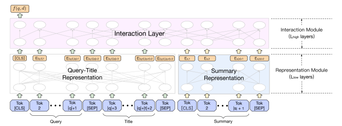 |
|---|
| Ranking Architecture |
The model is fine-tuned (the paper calls it pre-training, but I think it's more of a fine-tuning step) using triplet loss on a set of positive and negative pairs. The generation of positive and negative examples is covered below. Specifically, the PLM is fine-tuned to minimize the following loss:
Where refer to the true labelled score of documents respectively, and is the margin.
Relevance Score Calibration
Naively, we can curate using clicks and non-clicks respectively. However, the paper highlights several issues with this approach:
- Many clicks are in fact false positives, as they are caused by noisy clicks such as clickbait and accidental clicks
- There is exposure bias in the ranking system favouring higher position items
- Clicks do not necessarily imply relevance
Thankfully, there are many other signals accompanying each q, d pair, assuming that sufficient traffic has been observed for such a pair. Some examples from the paper include:
- , which measures the number of clicks vs number of users who were impressed but did not click.
- , which measures the number of clicks on the item as a fraction of all other clicks the user made for that query. This helps to control for users who are just trigger-happy and click on many items.
- , which measures the number of long clicks (i.e. user clicked and made no other action for
xseconds) against clicks.
These features contain signals about relevance that can be combined in a relevance model to infer the relevance of a q, d pair. To do this, Baidu crowd-sourced annotated ratings of a score from 0-4 for 70k query-document pairs. A simple decision tree-based model was then trained to infer the relevance score for a q, d pair given the relevance signal features discussed above. After training this model, it is then used to run inference on all q, d pairs (with sufficient observed traffic) to predict the relevance label and create a training dataset with a far more accurate relevance label.
Note: the paper also has a final step of fine-tuning the model according to crowd-sourced data, after the initial fine-tuning phase above with the calibrated relevance scores. Since this part is not particularly innovative nor feasible, I have omitted it here.
Experiments
They compared these innovations in an ablative manner from the original ERNIE system, which was a 12-layer transformer ranker trained using pairwise loss with human-labelled query-document pairs. The online ablation experiments show that:
- The inclusion of the document summary in the document representation adds around
0.65%in DCG@2 - The inclusion of fine-tuning on calibrated relevance scores increases the gains to
2.78%
The ablation experiments also showed that calibrated relevance scores is critical for effective fine-tuning. By using raw user clicks as signal, the positive-negative ratio (PNR, i.e. ratio of concordant q,d pairs over number of discordant q,d pairs) was only 1.86, but with the calibrated scores it increased dramatically to 3.35.
Takeaways
This is an interesting paper on building an effective pure search ranker (i.e. no personalization), although we can always layer additional personalization on top of the initial relevance score. The benefit of training a pure search ranker is that we can observe multiple instances of the same q, d pair, which allows us to bootstrap a diverse array of weaker relevance signals into a much stronger relevance score. Even if we do not have human-annotated signals to train the decision tree, we often have a sparser but stronger signal (e.g. conversion) and many other weaker but more abundant signals. Hence, it may be possible to use the same approach to predict the stronger signal from the weaker ones.
I suppose another way to deal with the diverse signal problem is multi-task learning, but this approach allows us to avoid the complexity of multi-task learning by first pre-processing relevance signals.
The idea of a on-the-fly query-sensitive document summary also sounds useful, and can probably be implemented with the help of ElasticSearch. We could extend this approach by performing query expansion before doing the document summary, which may allow us to fetch more relevant sentences which do not have exact term overlap. Another way of doing this is to pre-generate document summaries using an LLM, which requires assuming that one summary for a document is able to suit all queries, which may not be the case.
Dao 2022 - Flash Attention
This paper argues that the attention mechanism is slow because of reading / writing between GPU High Bandwidth Memory and GPU on-chip SRAM. The authors hence create a block-wise attention algorithm that minimizes such IO read / writes and speeds up attention significantly especially when the sequence length is long.
Brief Overview of Attention
Suppose we have an input sequence of embeddings where , such that . Naively, we can compute activations by , where , such that . However, this naive way of encoding our input sequence does not allow interaction between inputs at different positions (say with ). We can see this by observing that the first row of is only affected by the first column of (i.e. first encoding ), and likewise for all the other positions.
Attention addresses this problem by adding an interaction mechanism. Besides , we also create weight parameters . Given an input , we compute as follows:
We then create an interaction matrix , and apply row-wise softmax to get . can be thought of as a pairwise similarity matrix between the encoding at position and position that captures the degree of interaction. For example, in a sentence the economy has been in decline, the value of (assuming 0-index) measuring the interaction between economy and decline might be high.
Finally, we produce the output , which is an activation output from the input sequence that has captured the interactions between tokens at different positions of the input. This simple mechanism has led to significant improvements in language modelling.
GPU Memory Hierarchy
The memory hierarchy is such that read/write speed is super fast on the SRAM but memory is highly limited. Hence, the N x N attention matrix is written/read repeatedly to/from HBM, resulting in IO being a bottleneck. The numbers are as such on an A100 GPU:
- SRAM: 19 TB/s (20 MB RAM)
- HBM: 1.5 TB/s (40 GB RAM)
Naive Attention Algorithm
The naive attention algorithm has many reads and writes to HBM. (ps: Not sure why we cannot persist the intermediate matrices on SRAM and complete the computations, but in any case the naive algorithm requires materializing the matrices on SRAM which will quickly flood it. For example, a sequence length of 2,048 at float32 already takes up 33MB for the matrix).
- Load from HBM, compute , write to HBM
- Read from HBM, compute , write to HBM
- Load from HBM, compute , write to HBM
Flash Attention
The main idea is quite simple: instead of computing the full attention matrix, we use block-wise tiling to compute parts of it at a time. This reduces the memory required for each block and allows the whole computation to be done on SRAM while minimizing the amount of IO read from HBM, leading to faster compute time and lower memory usage on SRAM. The difficulty is in devising a block-wise softmax algorithm that yields the exact same result as computing it all at once.
Consider the naive softmax algorithm on an arbitrary vector .
Note that the maximum value is subtracted for numerical stability to avoid overflow (underflow is ok because ). is the numerator and is the sum of all elements in .
Now, the problem with the naive softmax algorithm in the context of attention is that we need an entire row of ( elements) to perform the row-wise softmax computation. This will not be available if we are performing block-wise computation, since we are splitting row-wise into blocks of . When we compute , blocks of will be materialized in each pass, but not the entire row at a time.
Hence, we need a modified algorithm that allows us to compute chunks of the final output at a time by iterating block-wise through , such that the combination of the new chunk of at each step with the already written intermediate gives the correct result at the end. The key to realizing this algorithm is in decomposing the softmax step, as shown below.
Consider two vectors . We can decompose the softmax of their concatenated vector as follows:
The first line of the above simply notes that the maximum of is the maximum over each of the subvector maximums . The second line notes that we previously multiplied each element of by a factor, say for those in . To get the correct multiplier for the full vector , we need to divide away the previous multiplier and apply the new multiplier, i.e. . The third line notes that the new denominator is the sum over each of the subvector sums, after we apply the correct multiplier from line 2.
The decomposition is simple but powerful. It implies that so long as we keep track of intermediate statistics and , we can compute the softmax of a long vector by splitting into subvectors and operate over each subvector at a time.
Now we are ready for Algorithm 1: Flash Attention of the paper.
Note that we use to denote a zero matrix of size and a zero array of size respectively. For simplicity, we divide into equal -sized blocks but the paper allows different block sizes for and . The equation numbers on the right in parentheses show which equations the lines correspond to above. Equation line 15 is a bit confusing because it combines multiple steps together. The next few paras try to unpack this.
Firstly, note that we are using the operator to denote an element-wise broadcasted multiplication. For a vector and a matrices , observe the associative property , since each element of only affects the corresponding row in the final matrix. This allows us to apply the scaling to either or and the result will be the same.
Next, see that the term is simply the corrected numerator of the softmax dotted with . Dividing this term by gives the output block for this particular pair.
Similarly, the other term is the existing output that has been accumulated from previous steps . Due to the associative property, we can also directly apply the scaling correction to . The are scaling factors according to equations (6), (8) to correct the scaling of previous steps.
Finally, we should understand why there is a + in equation 15. I find it easier to visualize if we set . If we trace the matrix multiplications, we will observe that is only affected by , i.e. it corresponds to only the query token in position . Now, represents the weighted average over all positions of the matrix where the weights are determined by the softmax over the interaction between (representing one token) and all positions on the matrix. This weighted average is why it is a symbol: we are accumulating the weighted sum over into . The only complication is that we are applying the scaling corrections at each step.
Hopefully these explanations provide some intuition to the FlashAttention algorithm, which is quite a simple idea but makes a ton of difference practically. It should be easy to implement this algorithm in numpy if the reader wishes to understand it better.
Wei 2022 - CoT Prompting in LLMs
Chain-of-Thought Prompting Elicits Reasoning in Large Language Models
This is an early paper that sparked the explosion of research on in-context learning for LLMs. The main idea is to use few-shot examples with the Chain-Of-Thought reasoning, i.e. <Question>, <CoT reasoning>, <Answer> , as opposed to just the question and answer alone <Question>, <Answer> (as per Brown 2020 - Language Models are Few-Shot Learners).
Method
The method is simple - we include the CoT reasoning in the few-shot examples included in the prompt, inducing the LLM to also generate CoT reasoning before answering the question at inference time. An example prompt:
Q: Roger has 3 balls. He buys 2 more cans of balls, each with 3 balls.
How many balls does he have now?
A: Roger started with 3 balls. 2 cans of 3 balls each is 6 balls.
3 + 6 = 9. The answer is 9.
What are some advantages of CoT prompting?
- Useable on black box LLMs. No fine-tuning is required, so we can readily apply it on off-the-shelf LLMs.
- CoT allows decomposition of complex problems into intermediate steps. The conceptual idea is that this allows the model to offload additional computation to the intermediate tokens, analogous to human reasoning.
- CoT reasoning offers interpretation of model behaviour. We have a suggestive trace of how the model arrived at that answer (though it would be naive to assume that the LLM uses the CoT trace reasoning exactly the way human logic operates).
Observations
An important sub-finding is that between CoT prompting and standard prompting (as per Brown 2020), CoT prompting's improvement gap significantly increases as we:
- Increase the question difficulty (seems intuitive); and
- Increase the model size. At the
8Bparameter model size, the study showed no difference between CoT prompting and standard prompting. But the gap widened significantly at the100Bmodel size and widened further at the500Bmodel size.
Another interesting ablation study tried to isolate the improvements to a specific aspect of prompting:
- Equation only. This would be something like
3 + 2 * 3 = 9for the above example. This showed to be no different from standard prompting. This showed to be useful on some datasets with simpler steps, but did not help on GSM8K which requires more semantic parsing of the question. - Variable compute only. One may argue that the exact tokens generated in the intermediate step does not matter much, all that matters is the additional compute the model performs to generate the intermediate tokens. Hence the authors prompt the model to generate dots
...as the reasoning step instead. This proves to not be helpful. - CoT after answer. Another argument is that including the CoT traces in the prompt improves in-context learning in and of themselves, meaning that the intermediate tokens are not actually necessary for improving the model's accuracy. The authors disprove this hypothesis by putting the CoT reasoning after the answer in the prompt, i.e.
<Question, Answer, CoT reasoning>. This forces the LLM to generate the answer before it generates the CoT trace. This also proves to not be helpful.
Thus the ablation studies help to clarify that it is the intermediate natural language reasoning steps that help the model offload computation and improve the accuracy of its answers.
Results
The performance of CoT few-shot prompting compared to standard few-shot prompting is striking:
- Using
GPT-3 175B, performance increases from15.6to46.9 - Using
PaLM 540B, performance increases from17.9to56.9
Honovich 2022 - Instruction Induction
Instruction Induction: From Few Examples to Natural Language Task Descriptions
This is an early paper that suggests taking a random subset of training (input, label) pairs, showing them to an LLM, and asking the LLM to guess the instruction that produces the label from the inputs.
Method
For example, the LLM prompt may look something like:
Here are the input-output pairs:
Input: As soon as you can.
Output: At your earliest convenience.
... (+4 more input / output pairs)
The instruction was ...
The LLM may then guess something like The instruction was translate the inputs into more formal language. We can then use this instruction as the new optimized prompt.
Note that this method is a one step process, i.e. it does not iterate for further improvements. But I suppose we can sample multiple random subsets of training instances and generate prompts for each before picking the best prompt based on execution accuracy on the validation set.
Evaluation
The paper found that the execution accuracy of these prompts with instruction fine-tuned version of GPT-3 (called InstructGPT) could reach similar levels to human-generated prompts on most simple tasks.
Notably, the authors were careful to control for the variation caused by the selection of few-shot examples:
- An
induce setof examples are held out from the training set - For each run,
5input / output pairs are randomly drawn from the induce set, and used to generate a prompt - The evaluation accuracy of this prompt is recorded
- The evaluation accuracy is averaged over
100runs
In hindsight, by using the idea of self-consistency, the performance can likely be significantly improved by taking the majority vote over the 100 runs rather than the average accuracy.
Huang 2022 - LLMs can Self Improve
Large Language Models Can Self-Improve
The main idea of this paper is that we can improve the instruction tuning of LLMs for reasoning capabilities using its own synthetic generated data.
Method
We are given a pre-trained LLM and a question-only training dataset (e.g. like GSM8k). We are also given a few-shot Chain of Thought examples (an example comprises of a question, a reasoning, and a correct answer).
The method is simple. For each question in the training set, we:
- Sample reasoning paths and answers
- Use majority voting from the answers to select the most consistent answer (this is called self-consistency in the literature). Importantly, to increase diversity:
- Set the temperature
- Apply mixed formats of prompts and answers
- Keep all reasoning paths that lead to as our synthetic dataset
- Fine-tune our LLM on the synthetic dataset using supervised fine-tuning
Note that since we are using self-consistency to obtain "labels" for our synthetic dataset, we do not require training labels.
Observations
For this method to work, self-consistency needs to be a reliable way of getting accurate answers. The authors plot the confidence score (% of paths leading to ) of against the accuracy at that confidence level, and find that it is highly correlated. This implies that highly consistent answers is a strong indication of correctness.
Generally performance increases as we increase the number of sampled paths . It seems to saturate at around . Also, the ideal temperature is around 1.2, showing that diversity is important for this technique to work well.
Findings
The fine-tuned LLM significantly advances the SOTA performance:
- GSM8K increases from
74.4using self-consistency to82.1(using self-consistency on the fine-tuned LLM)
Tunstall 2022 - SetFit
The task which SetFit tackles is few-shot labelling of texts. Since labelling data is scarce, current SOTA methods rely on large language models and techniques like In Context Learning (ICL) or Parameter Efficient Fine Tuning (PEFT).
Wang 2022 - Self Consistency LLM
Self-Consistency Improves Chain of Thought Reasoning in Language Models
The main idea of this paper is that majority decoding (dubbed self-consistency) of sampled LLM responses significant improves over CoT prompting (see Wei 2022).
Method
The idea is simple. As per (Wei 2022), we use CoT few shot examples in our prompt. Instead of just picking the answer from one run of the LLM, we sample many <CoT reasoning, Answer> pairs from the LLM with the same prompt. We then "marginalize out" the reasoning by just choosing the answer that occurs the most frequently.
Note that this method is unsupervised and the only cost to pay is the compute cost of multiple runs.
The name self-consistency comes from the idea that the most consistent answer given by the model is the most reliable one. Prior approaches to task-based responses is to use greedy decoding, i.e. set and get the highest likelihood answer. This paper shows that an ensemble of diverse answers is far more effective than the greedy approach.
We may think of this idea as analogous to random forests. Creating an ensemble over diverse weak learners improves significantly, and increasing the diversity of the learners (via column or row sampling) up to a certain point helps to improve performance.
Note that the idea of self-consistency decoding is orthogonal to the specific choice of CoT prompting. Specifically, self-consistency significantly improves with several forms of CoT prompting, including:
- Few shot in-context CoT prompts (Wei 2022)
- Zero shot
Let's think step by stepprompt (Kojima 2022)
Parameters
To generate diverse reasoning paths, the authors mainly refer to methods used in other papers:
- For
PaLM-540Bthey usedT=0.7andk=40with top-k token truncation - For
GPT-3they usedT=0.7without top-k token truncation
For the paper, the authors mainly sampled 40 paths.
Lee 2022 - RQ-VAE
Autoregressive Image Generation using Residual Quantization
Vector quantization VQ-VAE is used to represent an image as a sequence of discrete codes. After quantizing, an autoregressive model (AR model, e.g. transformer) is used to predict the codes.
This paper aims to reduce the sequence length of the discrete codes, as it becomes more computationally efficient for the AR model. However, reducing the sequence length (aka reducing the spatial resolution) causes a rate-distortion trade-off. The dilemma is such:
- Increasing the codebook size improves resolution of discretization to preserve quality
- But increasing the codebook size also increases the probability of codebook collapse, where only a subset of codes are used
The main idea of RQ-VAE is to reduce the spatial resolution by more precisely approximating the feature map at each location. Instead of increasing the codebook size, we use the codebook to recursively quantize the feature map in a coarse-to-fine manner. That is, the feature representation at each location is the sum of the selected codebook vectors at each level. For a codebook where each level has codebook vectors and levels, we can represent vectors for learning just vectors.
- The paper claims that due to this precise approximation, they can use just
8 x 8latents to represent a256 x 256image. That is a reduction of1024x!
Note: other papers usually use a distinct set of vectors for each codebook level, but in this paper they use a shared codebook for all levels. This is probably an implementation detail / hyperparameter to be tuned.
Method
There are two main stages:
- Stage 1: Residual Quantized VAE.
- Stage 2: RQ-Transformer.
Stage 1: Residual Quantized VAE
Let a codebook be a finite set be a codebook of tuples of a code k and its code embedding .
- is the codebook size
- is the code embedding dimension
Given a vector , let denote the discrete code of :
The normal VQ-VAE flow is such:
- Start with an input image , where are the original image dimensions
- The encoder extracts a feature map , where are downsampled times to form the latent feature map
- Applying the discretization independently to each position, we obtain a code map :
- We also obtain the quantized feature map :
- Finally, we decode the quantized feature map to reconstruct the image:
For Residual Quantization, we instead represent as an ordered tuple of codes:
Where is the discrete latent code of at depth . Specifically, we obtain by recursively quantizing the residual. Starting with residual , we compute the next as follows:
Finally, we represent as the quantized embedding of using the sum of embedding across all depths.
Note: by using a shared codebook and summing up the embeddings at each depth, this resembles bloom hashing (see Weinberger 2009). The difference is that we recursively / sequentially encode the residuals, whereas bloom hashing simultaneously applies multiple independent hashes and sums up those embeddings at the hashed positions.
However, as the experiments indicate, the embedding norms get smaller as we go deeper into the codebook levels, since it learns a coarse-to-fine encoding. So it seems to make better sense to have separate codebook vectors for each level.
The RQ-VAE flow is thus identical to the VQ-VAE flow above, except that the discretization step differs:
- Start with an input image
- Encoder extracts
- Discretize each position to get code map (note the additional dimension , since we now have codes per position):
- Finally decode:
RQ-VAE Training
The loss is:
The first loss is the reconstruction error of making the RQ-VAE roundtrip. The second loss is the commitment loss, which aims to push the encoder to reduce the quantization errors.
- Note that the commitment loss sums up the quantization error at each level of the codebook, not just the final quantization error at the end
- Also note that the authors did not include the loss to update the codebook as in VQ-VAE; instead they use the Exponential Moving Average approach to update the codebook using the average encoder output assigned to each cluster
Stage 2: RQ-Transformer
Given that we have learned a code map of , the goal is to now autoregressively predict the code map (laid out in raster scan order). Specifically, let us lay out into a 2D array of codes , where . Thus each row of (call it ) will contain codes:
Note that is laid out in raster scan order, meaning that we read the first row of pixels left-to-right, then move to the next row and so on.
Thus the goal of stage 2 is to learn an autoregressive model which learns the joint probability function , given all the prior tokens (i.e. causal masking). Note that we predict codes for each position before moving on to the next:
The natural approach is to just fit an autoregressive transformer decoder to this unrolled sequence (of length , where ). This incurs attention bottleneck complexity of . However, this paper argues that this is inefficient as it does not exploit the structure of our tokens, and proposes a customized RQ-transformer for this situation.
The idea is that there are two orthogonal dimensions, so we can decouple and create a specialized transformer to handle each one orthogonally:
- The first two dimensions, and , encode the position
- The last dimension, , encodes the depth
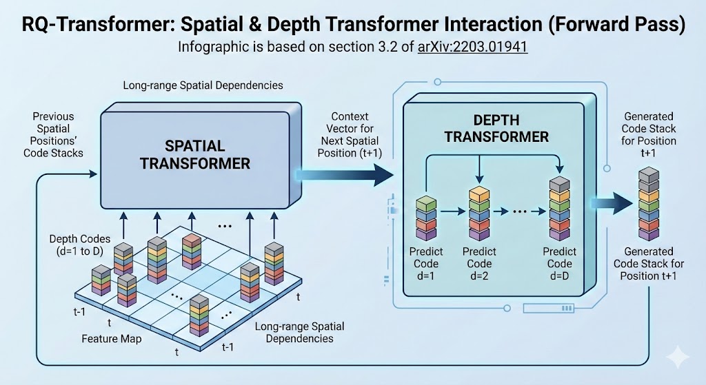 |
| RQ-Transformer Architecture |
Spatial Transformer
The spatial transformer encodes the position dimension and marginalizes away the depth dimension. It is concerned with the "big picture". Specifically, each input position to the spatial transformer is:
Note that:
- is the position encoding for spatial position
- We re-use the quantized embedding codebook vectors to represent inputs to the spatial transformer
- The depth position is marginalized out, such that we only need to encode positions with the spatial transformer
- is a special case for start of sequence and will have its own learnable embedding
The sequence of inputs is passed into a causally masked transformer to produce spatial context vectors like so:
Depth Transformer
Given the context vector provided by the spatial transformer, the depth transformer predicts a very short sequence of codes for this position . Thus, the depth transformer can be a smaller stack of transformer layers.
- Note: in the experiments, generally and in number of layers
Specifically, at spatial position and depth , input to the depth transformer is the sum of codebook embeddings up to depth :
The short sequence of inputs is passed into a causally masked transformer + classifier head to predict the codes for each position. The same depth transformer is reused across all spatial positions .
The autoregressive loss is simply the negative log likelihood of the correct latent token sequence:
Computation Savings
As observed above, fitting a naive transformer to the full sequence of length will incur attention complexity of . Compare this to the RQ-transformer:
- Spatial transformer: , since we marginalize away the depth dimension
- Depth transformer: , since we re-use the depth transformer times
- RQ transformer:
With , we have around 15x lower computational complexity:
- Naive approach:
4,194,304 - RQ transformer:
270,336 - Ratio:
~15x!
Other Tricks
There are two other tricks that they use in this paper, presumably to improve performance. The aim is to reduce the impact of exposure bias, which is the divergence between the samples during training and inference. During training, due to teacher forcing, we still get correct tokens to predict from at each position. During inference, since we generate each position autoregressively, errors can compound and lead the model to predict from a sequence that deviates far from what it has seen during training.
The main idea is to introduce some uncertainty into both the labels and inputs to the training process. Let us define a categorical distribution on conditioned by the encoder embedding , with probability distribution:
Thus the probability of a discrete token increases exponentially as its quantized embedding gets closer to the encoder embedding . Note that as approaches , gets sharper and converges to the one-hot distribution .
This soft approximation of the argmin is used for soft labelling of the objective when training the RQ-transformer. Specifically, note that at position and depth , we quantize by doing a nearest neighbour search for the residual vector . Hence the hard target for the RQ-transformer training is the one-hot label . Instead we replace with .
We also do Stochastic Sampling of the latent codes when generating training samples for the RQ-transformer. Instead of deterministic code selection when encoding the raw images to latent codes, we sample from the categorical distribution of .
The ablation studies show that using soft labelling + stochastic sampling significantly improves performance.
Results and Hyperparameters
General hyperparameters:
- Codebook size:
- Codebook levels:
- Latent dimension size:
- Temperature:
Generally RQ-VAE matches or outperforms image generation of other autoregressive competitors like VQ-GAN. It is also a lot faster in generation speed and memory usage.
Tay 2022 - Differentiable Search Index
Transformer Memory as a Differentiable Search Index
This paper proposes a new paradigm of search. Instead of using Approximate Nearest Neighbour (ANN) search using embeddings, the paper proposes to train a transformer seq2seq model to predict the ID of a document given a search context.
Although the paper is focused on search and Question-Answering, the approach is general and can be used for any recommendation setting.
Comparison to Traditional Search Index
Traditional search index such as BM25 or ANN search has three steps:
- Indexing. Indexing involves storing representations of each document to enable easy search later on. For traditional lexical search like BM25, a sparse and high dimensional vector is stored for each document and an inverted index is built. For ANN search, a dense vector is stored and an index like HNSW is built.
- Training. For lexical search, the only "training" is to store the TF-IDF quantities in the index. For ANN search, a contrastive learning objective is used to shape the embedding space for effective retrieval.
- Retrieval. For lexical search, a lookup of the inverted index based on the query terms is performed. For ANN search, a Maximum Inner Product (MIPS) search is performed using some algorithm.
The differentiable search index operates differently. The authors argue that it is more elegant:
- Indexing. Indexing is just a specific form of model fine-tuning. Specifically, the task is to predict the
docidgiven thecontentof the document, i.e.f(doc_content) = docid.- There is no need to store a separate search index as the only artifact we need becomes the transformer model itself
- Training. Training is a form of supervised fine-tuning where we predict
f(query) = relevant docid. - Retrieval. Retrieval is simply running a forward pass on the transformer on a new query.
The nice thing about this setup is that it extends naturally to a multi-task setting, by using different prefixes for different tasks. This is similar to the T5 approach for multi-task learning.
Ablations
The main idea is simple and intuitive, but there are many details to the implementation that are non-trivial.
Indexing Strategy
The indexing step aims to teach the transformer model how to link each docid with the contents of the document. This is entirely new knowledge to the transformer since the docids are arbitrary constructs.
The following strategies were explored:
f(document context) = docid: this had the best performancef(docid) = document context: this performed terriblyMix of 1. and 2.: Mix training batches with both options1and2, with a prefix string to indicate which direction.
Indexing and Training Order
Recall that we have two modes:
- In indexing mode, our training data is
f(document content) = docid - In training mode (or retrieval task), our training data is
f(query) = relevant docid
The following strategies were explored:
Index first, train second. This means that we train with the indexing mode until convergence, then switch to training modeMulti-task. This means that we mix training batches of both indexing mode and training mode and just use a prefix to indicate the different task setting
The multi-task strategy worked much better. The performance was sensitive to the mix between indexing and retrieval task. The ideal mix was found to be around 32 instances of indexing task to 1 instance of retrieval task.
Representation of Document IDs
The following strategies were explored:
-
Arbitrary Atomic Identifiers. This means assigning an arbitrary random identifier for each document, and letting each identifier be a new token in the vocabulary.The downside is that there is an explosion in the vocabulary if we have a lot of items
-
Semantically Structured IDs. This means representing each document as an ordered list of tokens, where the tokens contain some semantic meaning.This is implemented as a hierarchical k-means clustering.
- Firstly, each document is embedded using a universal T5 embedder.
- Next, k-means with
10centroids is performed. The cluster ID0-9is assigned as the first document ID token for each document - Each cluster is then further clustered to generate the subsequent document ID tokens
Inference Time
To generate recommendations at inference time, given a query, we pass it into the transformer model and just do generative decoding with beam search. Beam search maintains at each decoding step top k candidates based on log probability. The top k candidates sorted in descending log probability is thus our list of recommended candidates.
Results
Overall, the semantic ID approach was the best performing, and had significant gains over a fine-tuned dual encoder model.
The scaling effects of larger models seemed much better with the DSI approach compared to dual encoders. In my experience, dual encoder models also don't seem to benefit much from scaling to larger models (minimal effect scaling from 20M models to 500M models.)
The DSI approach is closer in performance with hits@10 to dual encoder but had much better hits@1 performance.
Concerns
One finding was that shorter representations of the document (truncate at first L tokens) worked significantly better. The authors suggested that longer document lengths might make indexing memorization more difficult. This seems like a significant bottleneck to the paradigm, but future work might resolve this issue.
One big shortcoming of this current method as-is is that the embedding representation used is an OTS T5 model. Subsequent papers will find that relevance-based fine-tuned embeddings perform much better at generating good semantic IDs to represent each document.
Rafailov 2023 - Direct Preference Optimization
Here we trace the derivations from the DPO paper. Denote the model after SFT as , i.e. the policy is a probability function for each pair of inputs and answers (x, y). Naturally, we can use this policy to generate tokens by choosing the response with the highest probability (or approximate it in a greedy token-by-token manner).
To perform RLHF, we first need to build a reward model. First, we prompt the SFT model to obtain pairs of answers . These samples are presented to human labellers who record their preferences in the form , where wins and loses. These preferences are assumed to be generated from an underlying reward model which we do not have access to.
We wish to learn this reward model. Since we only have access to pairwise preferences instead of the reward score, a common approach is to model the pairwise preferences using the Bradley-Terry model. Specifically, we assume that the observed human preference decisions are related to the underlying human reward model in the following way:
Suppose we have a static dataset of comparisons sampled from the human preference model of . We can create a reward model and use the BT-model to express the negative log likelihood of . Note that are we using the expression of the BT-model as a sigmoid function. With this NLL expression, we can optimize for using gradient descent to learn the reward model from . Notice that the heart of Equation (2) is essentially just a difference in reward between the winning answer and losing answer .
Note that is usually initialized using the SFT model , but with an additional linear layer over the final transformer layer to generate a scalar value as the reward.
Having learned the reward model, we then need to use the learned reward function to fine-tune using reinforcement learning. Specifically, we set as the reference model, and initialize a new model that we wish to train. Usually, is also initialized as a copy of . The objective function we wish to maximize is:
Inspecting this objective, we see that we are trying to tune such that it generates answers that maximize the learned reward function , while at the same time ensuring that we do not deviate too far from the original reference model. is a hyperparameter controlling the degree of deviation. This penalty constraint serves to:
- Ensure that we do not drift too far from the
(x, y)distribution on which the reward model is accurate - Ensure that we maintain generational diversity and not just collapse into a single high-reward answer for a given prompt
Objective (3) may not be directly optimized, because we need to generate at each step from the current policy (not sure if I fully understand this). Hence typically this is optimized using reinforcement learning using PPO.
Direct Preference Optimization
The RLHF process in general is unstable, requires more memory / computation and requires tricks to make it work. Hence the authors of DPO set out to create an optimization procedure that:
- Avoids fitting an explicit, standalone reward model
- Avoids using reinforcement learning
DPO starts off with the KL-constrained reward maximization objective from Equation (3) above. The first step is to show that the optimal policy for this objective is of the following form for an arbitrary reward model :
The derivation for Equation (4) is as follows. For a given reward function :
For line 2 above, recall that is the expected value of if the random variable is drawn from . Since the outer expectation is over draws from , we can breakdown the KL-divergence by bringing the log difference into the expectation. Line 3 simply divides by and flips max to min. Line 4 uses to bring the reward term into the denominator of the left term, then introduces an arbitrary . Note that the two can be cancelled out if we brought them together, but we will be using them later on.
Now let us define the optimal policy . We will need to prove that is indeed optimal. Note that is a valid probability distribution as:
- ; and
- , since the denominator is just the sum over of the numerator
Since is not a function of , we can sub in and take out. The left term becomes a KL-divergence between which we are optimizing over and the optimal policy .
Finally, note that does not depend on , so we only need to consider the KL-divergence term. Gibb's inequality tells us that KL-divergence is minimized at if and only if the two distributions are identical. This completes our derivation of (4) by showing that is indeed the optimal policy.
Now that we have completed the derivation, let's consider what Equation (4) is saying. It tells us that we have an analytical solution for the policy that optimizes (3), and that it can be expressed in terms of (which we already have) and a given reward function .
Since we previously learned a reward model , we could simply plug that into (4) to get our optimal policy. Specifically, for a new input prompt , we can compute for all possible values of and pick the best . We can ignore since it is fixed for a given prompt . Intuitively, the new model scales the probability of high reward answers up with an exponential multiplier, and the degree of scaling is controlled by . However, this is not computationally practical as we need to evaluate over a very large space of (i.e. all possible answers for a given prompt ).
Hence, we want to find a form of the optimal policy which does not involve the partition function nor the reward model . We start by re-arranging Equation (4), taking log on both sides and re-arranging:
Since Equation (5) holds for any arbitrary reward model, we can use the optimal (unknown) human reward model back in Equation (1), . Also, note that in Equation (5) refers to the optimal policy under , so since we are using the optimal reward , we can call this optimal policy as well. Now we plug Equation (5) back into Equation (1).
The derivation of the above is quite simple, we just need to note that it is of the form , and use the expression of the BT-model as a sigmoid function. The great thing is that the pesky partition function cancels out because the BT-model simply ends up with the difference between two scores / rewards.
Equation (6) looks simple but is quite remarkable when we compare it to Equation (1), because we now have the probability of the human preference data in terms of just the reference policy and the optimal policy , without the reward model at all! Of course, the reward model is implicitly embedded in the equation. If we stare at Equation (6), we see the implicit reward function is .
The benefit of this new formulation is that we can write the maximum likelihood objective in terms of the optimal policy. We do not know the optimal policy, but we can parametrize it as and use the maximum likelihood objective to train the model. Our new policy objective becomes:
Application to Dual Encoder Retrieval
The DPO framework offers a way to fine-tune a policy according to human preferences, whilst ensuring stability against a reference model. In the original formulation, represents the probability of generative model generating given an input prompt .
A related problem is that of fine-tuning embedding models for search retrieval, in what is known as the dual encoder framework. In this case, we also have preference data in the form of triplets (query, positive_passage, negative_passage), and we wish to fine-tune embeddings such that the dot-product or cosine similarity between (query, positive_passage) is high whilst that of (query, negative_passage) is low. In this formulation, we could let the policy represent the normalized probability of a relevant match between query and passage. We can then borrow the framework of DPO to fine-tune our embeddings. The benefit of DPO compared to typical optimization objectives for dual encoder is the stability of the policy against the reference policy, which hopefully is a good form of regularization even when preference data is limited.
Specifically, we define a dual encoder policy , where represents a query and represents a passage, like so:
- Encode into a vector using a BERT model
- Encode into a vector using a BERT model (can be same model as the query encoder)
- Take the dot product
- Run the dot product through a sigmoid layer to convert it into a probability
We can then apply this method to a reference encoder model and call it , and optimize another encoder model against this reference model. Will need to conduct experiments to see if this method offers gains against the typical dual encoder objectives, such as Karpuhkhin 2020.
References
Blecher 2023 - Nougat
Blecher 2023 - Nougat: Neural Optical Understanding for Academic Documents.
Nougat is an end-to-end system that converts a scientific PDF into a sequence of tokens in markdown format in an auto-regressive way.
Prior methods for Visual Document Understanding (VDU) usually rely on an external OCR service to generate intermediate outputs. In contrast, this method is end-to-end, and the text is generated directly from image embeddings in a decoder manner. Thus, the model is very simple and most of the work in this paper is in data preparation.
Model
- Encoder. The encoder gets a variable size document image and applies crop / resizing to generate a fixed rectangle of size . Smaller images are white padded. The fixed size image can then be passed into a Swin Transformer to output a sequence of embedded patches where is the latent dimension and is the number of patches.
Dong 2023 - MINE Loss
Revisiting Recommendation Loss Functions through Contrastive Learning
This paper compares several recommendation loss functions like BPR, CCL and introduce two new losses: InfoNCE+ and MINE+.
Setup
Let denote the user and item sets. We denote that:
- Each user has interactions with items, and has no interactions with the remaining set of items.
- On the item side, denotes all users who interacted with item
- We can also denote if there was an interaction and otherwise
Let the latent embeddings represent user and item respectively. The similarity measure between them is then denoted .
BPR Loss
The most widely used loss is Bayesian Personalized Ranking:
Note that for each user, we take the expectation over the set of items relevant to him. We then sample negatives from the overall item distribution (usually uniformly at random).
Softmax Loss
One common approach is to model as an extreme classification problem where is a very large set. The probability may then be modeled as a softmax:
In practice, it is infeasible to compute over the large item set, so we sample negative candidates for the denominator. The sampling is then corrected via importance weighting.
- Covington 2016 for such an approach.
- Jean 2014 for importance weighting correction
Using this approach, the loss may be formulated as:
Note that is a negative sampling distribution for each user , and is typically implemented as which is based on item popularity.
Contrastive Learning Loss (InfoNCE)
InfoNCE loss looks very similar to the sampled softmax loss, although the motivation is different. The key idea is to pull similar points closer and push dissimilar points apart. InfoNCE loss is the most famous contrastive learning loss:
Note that the only difference from the sampled softmax loss is that the is inside the sum rather than outside. The InfoNCE loss has been shown to maximize the mutual information between user and item and minimize mutual information between unrelated pairs.
Empirical Exploration of InfoNCE+
The authors propose an InfoNCE+, which is just adding some hyperparameters to InfoNCE and performing some empirical tuning of these hyperparameters. The InfoNCE+ proposes adding and :
Empirically, the authors find that setting and usually works best (tbh, the empirical evidence is not super convincing).
Theoretical Support for Removing Positive term from Denominator
As we can see, setting effectively removes the positive term from the denominator of the loss. This makes intuitive sense as it would constrain from increasing which is what we want.
This has theoretical backing as well, as explored in Decoupled Contrastive Learning - Yeh 2022. The DCL paper also shows that removing the positive term from the denominator leads to more stable training and less hyperparameter sensitivity.
The DCL loss is thus:
The authors also show that this "decoupling" is also justified from the Mutual Information Neural Estimator perspective. Specifically, the MINE paper shows that we can estimate the true mutual information between each user and item by the following optimization problem:
Intuitively, we want to maximize the above equation over the similarity function parametrized by the embeddings .
- The first term takes an expectation of similarity scores over the joint user, item distribution where an interaction occurs (i.e. positive pairs).
- The second term takes an expectation of exponentiated similarity scores over the product measure of marginal user and item distributions (i.e. assuming independence between user and item distribution).
MINE Loss
The authors then say that a "simple" adaptation of the MINE problem to the recommendation setting is formalized as the MINE loss:
Not too sure how this is derived from the above.
They also add a hyperparameter to control the relative weightage of the positive and negative samples. This results in what they term as MINE+:
Based on some ablation studies, they find that usually works best.
The paper also offers some lower bound analysis and de-biasing of InfoNCE which I will not delve into for now.
Liu 2023 - Meaning Representations from Trajectories
This paper demonstrates a way to compute sentence similarities using auto-regressive LLMs with a decoder-only architecture.
In the encoder-decoder setting, characterized by BERT models, a sentence is typically represented by the embedding generated by the encoder at the final layer. Typically, either the [CLS] token embedding is taken, or the element-wise mean of the embeddings at the final layer is taken to represent the sentence. As Reimers 2019 demonstrates, the default BERT trained using masked language modelling objective does not automatically have good embeddings suitable for Semantic Textual Similarity tasks. Hence the BERT model needs to be fine-tuned with some sentence similarity training task to generate good embeddings.
This paper is interesting as it does not require any such fine-tuning. The main idea is to represent a sentence (sequence of tokens) by the distribution of text continuations (denoted as trajectories) generated by the auto-regressive LLM on the context sentence. In other words, as the paper elegantly puts it, we represent the meaning of linguistic terms by their usage.
Setup
Let denote a finite vocabulary of tokens and indicate the set of all variable-length finite sequences of tokens in . A language model may be viewed as a map that associates a prompt sequence and a possible continuation sequence with a likelihood score .
The paper chose inverse perplexity as the score:
Side note on inverse perplexity. We know that perplexity is as below. Hence the above score is indeed the inverse perplexity.
Given two prompts and , we denote their semantic representation under model as and . The semantic distance between them may be denoted where is some distance function. The paper chose:
In other words, we sample a continuation trajectory with equal probability from either prompt and generate a continuation sequence of length m, and compute the expected difference in log-likelihood of the generated continuation between the two models and . Since it is not feasible to integrate the above expression over all possible trajectories , we sample trajectories and compute an estimation to the above expected difference.
Results
For the experiments, the authors set n=20, m=20, and sampling temperature =1.0.
- Ablating on number of trajectories
nshows that most of the performance is achieved withn=20, with marginal gains thereafter - Ablating on sequence length
mshows that most of the performance is achieved withm=20, with marginal gains thereafter. Interestingly, there is a big improvement in performance fromm=1tom=10, showing that the distribution of the next token alone is not sufficiently discriminating as a semantic representation. - Ablating on sampling temperature shows that
1.0is optimal. Sampling from too diverse or too similar trajectories hurts the performance of this method.
The results show that this method is the best way to represent autoregressive models thus far, with even slightly better performance than encoder-based models like T5 on the STS task. The results are not as good as models explicitly trained with unsupervised contrastive learning (see SimCSE) for the STS task, but as the decoder model size is increased, the performance starts to reach similar levels.
Application to Semantic Retrieval
Unfortunately, this method is not suitable for semantic retrieval, as the distance measure requires sampling from both query and document distributions (if we treat query as one prompt and document as the other prompt). Note that the setting is Semantic Textual Similarity where query and documents come from similar distributions.
The authors create a proof-of-concept workaround by creating a fixed set of trajectories that is used instead of sampling , where they select random documents from the dataset and create a sample trajectory from each document to form . We can then precompute for each document on this set of trajectories . At inference time, we just need to compute on the fixed set of trajectories, then compare the distance against the pre-computed to get the distance scores. The authors show that this approximation obtains reasonable performance.
However, I note that in typical semantic search settings, query and document usually come from different distributions where queries are short and documents are long. Hence, the continuations of a query and document might not be directly comparable. However, the beauty of this method is that since it is based on continuations, we can use prompting to adjust the behaviour of the LLM to somewhat align distributions.
For example, we may on the document-side generate trajectories using a prompt like Given document d, generate a query. On the query-side, we may use something like Given query q, generate other similar queries. We can then compare trajectories generated in this fashion.
Another issue with the original workaround is that of latency. Even with a fixed trajectory set, we need to compute at inference time, which is costly even for small number of trajectories. One way to deal with this issue is to have a hybrid setup:
- On the
documentside, we use the high-precision decoder to generate a prospective set of queries from documents of sizen(sayn=1,000). Each document is represented as a embedding of sizenwhere each position records the likelihood of prospective query given document using the decoder model. - We use a separate fine-tuned encoder model to precompute embeddings for each of the prospective queries.
- On the
queryside, during inference, we use the same encoder model to embed the query and compute similarity against thenprospective queries. The similarity scores form a representation of sizenfor the query. - We may then compute similarity between the size
nquery and sizendocument representations and perform retrieval with standard nearest neighbour vector databases.
In contrast to standard embedding vectors where each position encodes an unknown quality, these representation vectors have clear semantic meaning in each position (indicating the strength of relation to a particular prospective query). This setup also allows us to trade-off precision against recall by tweaking the sparsity of the representation vectors using score thresholding or top-k thresholding on either (or both) the query and document side.
Klenitskiy 2023 - BERT4Rec vs SASRec
Turning Dross Into Gold Loss: is BERT4Rec really better than SASRec?
This is a short paper that argues the alleged performance gains of BERT4Rec over SASRec is not due to the masked cloze prediction task and bi-direction attention as the authors claim, but rather due to the loss function.
BERT4Rec uses softmax cross entropy over the entire item catalog at each time step, whereas SASRec uses binary cross entropy against a single sampled negative at each time step. When the same softmax cross entropy is used for SASRec, it outperforms BERT4Rec consistently and trains faster.
Background
Sequential recommendation is a popular approach currently to recommender systems, and in particular transformer models with self attention are the standard approach. SASRec is the standard approach, where the task of sequential recommendation is treated as a causal modelling task where the self attention mechanism is only allowed to attend to previous time steps when making the prediction at time step .
BERT4Rec was proposed as an improvement to SASRec, and the claim was that introducing bi-directional attention (like BERT) and performing prediction on the cloze passage task (i.e. randomly masking x% of items) is able to lead to significant gains over SASRec. The argument is that the random masking is akin to data augmentation, as there are far more permutations of masked positions compared to just predicting the next item.
The authors point out two misgivings they have with this interpretation, which is in line with my own intuitions:
- BERT4Rec task is only weakly related to the final goal of sequential recommendations, whereas SASRec tasks for training and prediction are perfectly aligned (i.e. just predict the next item). This is akin to only using the BERT encoder (without the decoder) for a language modelling task, which is quite strange.
- BERT4Rec masks some items and only calculates losses for the subset of items, whereas SASRec computes losses for all items (except the last item) at once, getting more training signal from each training sequence
So we should expect SASRec to perform better and more efficiently than BERT4Rec. How then do we explain the performance discrepancy? The authors hypothesize that the performance difference is really due to the difference in loss functions between them, as explained below.
Setup
Start with a set of users and items . Let each user be represented by a sequence of item interactions . Each sequential deep learning model may be abstracted as an encoder of input sequence , and the encoded sequence be denoted , where is the latent dimension.
To make predictions, given the full item embedding matrix , we take:
Then the element of may be denoted as represents the predicted relevance of item at time step for user .
SASRec: Binary cross entropy loss. SASRec does not compute the full prediction matrix. Instead, for each true positive item at each time step, it randomly samples one negative item and computes the predictions and . Then the loss is:
BERT4Rec: Softmax Cross Entropy. In contrast, BERT4Rec computes the full prediction matrix for each user and computes the softmax over the entire item catalog for each masked item prediction. The cross entropy loss is thus:
Note that for BERT4Rec, the inner summation is only over the time steps with masked items. If we were to translate this loss to SASRec, we would sum over all time steps.
Sampled Softmax. Finally, it may not be computationally feasible to compute the softmax over the full item catalog. Hence the authors propose that for each user sequence in a batch, we sample items a user has not interacted with and use the same set of negatives for each time step of a given sequence. Let denote all items that user has not interacted with. The loss is then:
Qn: This means that we have a different set of negatives for each user in a batch? Seems quite memory intensive.
Experiments
The authors use the full sequence of item interactions for each user. The last (most recent) item is held out as the test set, and the second last item is chosen as the validation step. Models are trained with early stopping on the validation set. The authors note that the common practice of sampling negative items for metric computation is not a robust one, as it introduces randomness into the metrics.
Note: I think the other reason sampling negatives is not robust is because it does not directly mirror the retrieval task, which requires choosing an item from the full catalogue.
The results show that SASRec with 3,000 negatives is consistently the best model, beating BERT4Rec consistently. It also trains around to times faster than BERT4Rec. Hence the authors recommend sampled softmax SASRec as the de-facto standard instead of BERT4Rec.
The authors do note that for the smaller datasets, SASRec may overfit relatively quickly (validation loss peaks and declines) and hence it is important to use early stopping. In contrast, BERT4Rec is more robust to overfitting and validation performance generally does not decline (it plateaus near the peak).
Singh 2023 - Semantic IDs for Recs
Better Generalization with Semantic IDs: A Case Study in Ranking for Recommendations
This paper proposes uses semantic IDs instead of hashing to random IDs to represent user or items. Semantic IDs mean that collisions to the same ID are semantically meaningful, and hence addresses the collision problem and also offers better generalization in cold start scenarios. The paper shows that this approach (i) retains memorization ability on par with random hashing and (ii) generalizes much better to unseen items and (iii) is much more computationally efficient as each user / item is represented simply by a 64-bit integer.
Background
In industry recommender systems, users or items are typically represented using random bloom hashing on a string ID (see Weinberger 2009) into an embedding table. Such IDs have no semantic meaning, so collisions in this approach degrade performance. Nevertheless, it is empirically clear that the item-level memorization is important for good recommender performance. On the other extreme, one may choose to avoid IDs entirely and simply represent items using their content embedding. While it is clear that this obviates the collision problem and improves cold-start performance, multiple papers have shown that performance will be degraded overall due to inability to match the memorization ability of ID-based recommenders.
The ranker used in experiments is from Google's video recommender. See Improving Training Stability for Multitask Ranking Models in Recommender Systems and Recommending What Video to Watch Next: A Multitask Ranking System.
Approach
The approach pre-supposes that every item (video in this case) already has a good learned embedding. For Google's case, they have a video encoder that represents each YouTube video as a 2048 dimensional vector that captures the topicality of the video. The encoder takes both audio and visual features as input. The model training is described in Large Scale Video Representation Learning via Relational Graph Clustering.
The approach has two stages:
- Represent each item as a sequence of Semantic IDs. They employ a method called RQ-VAE to compress a dense content embedding into a few discrete tokens (represented as integers) which capture the semantic content.
- Train the ranking model with Semantic IDs. Once trained, the RQ-VAE model is frozen and used to generate semantic IDs for each item. We then train embeddings for each semantic ID along with the rest of the ranking model.
Stage 1: RQ-VAE for Semantic IDs
The idea of RQ-VAE is to iteratively find tokens that match the content embedding. Once a token is found, the next token will try to match the residual embedding and so on.
Let be the content embedding. The algorithm is as follows:
- Use encoder to map the content embedding to a latent vector
- The residual quantizer of layers recursively quantizes into semantic IDs
- Each level has a codebook containing vectors (
K=2048in this paper) - The residual for level is used to find the nearest codebook vector
- The ID associated with is taken as the semantic ID
- We compute
- Thus we end up with a sequence of semantic IDs (e.g.
(1, 4, 6, 2))
- Each level has a codebook containing vectors (
- A decoder maps the quantized latent back to
The RQ-VAE model is trained with the following losses:
- aims to reconstruct the content embedding
- where is the stop-gradient operator (which disables gradient updates to the term in the operator). This is to encourage and the codebook vector to move toward each other, so that we have a good codebook at the end.
Stage 2: Using Semantic IDs for Ranking
Now that each item is represented by a sequence of semantic IDs , we can treat each ID as a token. The most intuitive thing is to treat each token as a subword and assign a unique embedding to each token (this is the unigram approach below). Unfortunately, this simplistic approach is not the most ideal. The experiments reveal that these semantic tokens behave more like characters in NLP, and it is important for performance to assign unique embeddings to sequences of tokens (i.e. create subwords out of the characters).
There are two approaches that were experimented:
- Create n-grams out of the IDs. Suppose an item has semantic IDs
(4, 6, 3, 2). A unigram approach would look up embeddings for each ID by itself. A bigram approach would look up embeddings for(46, 63, 32)and so on. Consequently, the embedding table size for a quantizer withLlevels andKcodes in each level is something like . This gets prohibitively expensive for largerN, so the experiments stop at bigram. - Sentence piece based. As with natural language, most n-grams rarely occur (or do not occur) at all. Hence the n-gram approach is wasteful. The authors found that applying the sentence piece approach (I suppose using byte pair encoding?) is an effective way to learning the subwords to assign a unique embedding. The authors train the subword model on impressed items to a desired arbitrary vocab size. Note: this makes the approach less flexible, as we need to freeze both the quantizer and the set of subwords. However their experiments show that this is generally quite resilient.
Results
The experiments use CTR AUC as the target metric. The model is trained on a window of N days and predictions on day N + 1. Cold start performance refers to the performance on the subset of items that were newly introduced on day N + 1. Note that each user is represented as a sequence of items, including past item history and the current item. The item is represented by semantic IDs for itself. The main findings of the experiments:
- Sentencepiece (SPM) approach > n-gram approaches for overall performance. As the vocab size is scaled up for the
SPMapproach, it outperforms both unigram and bigram easily. - SPM > random hashing with the same vocab size for overall performance. It does not compromise on the memorization capacity of the model.
- All Semantic ID approaches > random hashing in the cold start scenario (as expected)
The authors also conducted a set of experiments where items are represented by their content embedding directly. Due to the large size of the embedding, they did not include user past history for these experiments. These showed that content embedding approach is inferior to random hashing, unless the number of layers is increased significantly. This suggests that a larger model is indeed able to memorize better just using the content embeddings, but at a significant computational cost. Hence this justifies the use of semantic IDs as a more efficient way to balance between memorization and cold start performance.
Takeaways
Semantic IDs is a promising approach to balance memorization and cold start performance. However, it presupposes that we have good embeddings for each item. It also introduces significant engineering complexity in training and freezing a residual quantizer and a fixed subword vocabulary. Although the authors conduct experiments to show that this quantizer is quite robust to data distribution shift, there would probably come a time when we need to update the quantizer and the subword vocabulary and deal with the refreshing issue.
Yang 2023 - OPRO
Large Language Models as Optimizers
This paper proposes an automated prompt optimization technique that resembles optimization. Compared to previous efforts, this paper makes use of an LLM's ability to understand patterns and what they call optimization trajectories to optimize a prompt.
Method
We have access to a training set of <question, answer> pairs. The idea is simple:
- Test out a prompt with the task description and evaluate the accuracy
- Append previously tested prompts and its accuracy in an ascending score order (keeping only the best
8prompts in the trajectory) - Ask the LLM to write a new prompt that is different from the old ones and achieve a high score
Motivation
The authors motivate this by showing that LLMs can solve simple linear regression and travelling salesman problems. For linear regression:
- A true generating equation of is chosen
50data points are generated with gaussian noise- The goal is to get an LLM to guess what is the best
(w, b)pair - The algorithm loops through the following:
- Start with
5random(w, b)pairs, compute their mean-squared error - Prompt the LLM with these pairs and tell it to suggest
8new(w, b)pairs that further reduces the loss - Evaluate the MSE of these new pairs and replace the pairs in the history
- Keep up to
20pairs in history
- Start with
It is not obvious that LLMs can accomplish this task, as it requires some understanding of the underlying generating equation and how to nudge the w, b values. However, the paper shows that LLMs can generally solve this task and reach the global optimum, and that better models (e.g. gpt-4 vs gpt-3.5) achieve the optimum in fewer number of steps.
OPRO for Prompt Optimization
The general layout of a prompt is like so (note that the Comment
headers are not part of the prompt):
### Comment: Meta Instruction for Optimization Trajectory ###
I have some texts with their corresponding scores. The texts are arranged in ascending order based on their scores, where higher scores indicate better quality.
### Comment: Optimization Trajectory ###
text:
Let's figure it out!
score:
61
... more history ...
### Comment: Meta Instruction for Few Shot Exemplars ###
The following exemplars show how to apply your text: you replace <INS> in each input with your text, then read the input and give an output. We say your output is wrong if your output is different from the given output, and we say your output is correct if they are the same.
### Comment: Few Shot Exemplars ###
input:
Q: Alannah, Beatrix, and Queen are preparing for the new school year
and have been given books by their parents. Alannah has 20 more books than Beatrix. Queen has 1/5 times more books than Alannah. If Beatrix has 30 books, how many books do the three have together?
A: <INS>
output:
140
... more exemplars ...
### Comment: Final Meta Instruction ###
Write your new text that is different from the old ones and has a score as high as possible. Write the text in square brackets.
Optimization is tested out on GSM8K (grade school math problems) and Big Bench Hard (logical reasoning questions). At each step, the above prompt is used 8 times to generate 8 different prompts. These prompts are evaluated on the training set. The best scoring 20 prompts are kept in the optimization trajectory at any point in time. Other parameters:
Temperature = 1when generating prompts for diversityTemperature = 0when evaluating each prompt on the training set with the scorer LLM for greedy decoding
The optimization trajectory looks like this, resembling actual optimization.
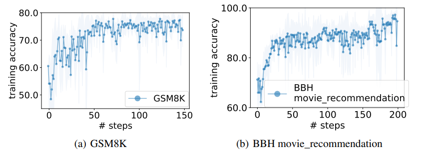 |
|---|
| OPRO Optimization Trajectory (Figure 1 from paper) |
Notes
The method is intuitive and compelling. The downside is that inclusion of both optimization trajectory and exemplars makes the method quite costly, although the optimization only needs to be done once to get the best prompt.
Rajput 2023 - Generative Retrieval
Recommender Systems with Generative Retrieval
Borisyuk 2024 - GNN at LinkedIn
Borisyuk 2024 - LiGNN: Graph Neural Networks at LinkedIn
This is an applied paper documenting learning points from LinkedIn's latest Graph Neural Network (GNN) models, geared toward industry practitioners.
The main architecture is based on GraphSAGE. The graph is heterogenous, where nodes can represent a company or member or post etc., and edges can represent (i) engagement of a user with a post, (ii) affinity between a member and a creator, and (iii) whether a member or company has a particular attribute. Edges are weighted by the strength of the engagement, except attribute edges which all have a weight of 2.0.
The GNN's are trained as encoders for the various types of nodes, and the generated embeddings may be used for downstream link prediction tasks. They are trained using the GraphSAGE framework, which inductively generates the node embeddings using graph sampling and neighbourhood aggregation. The graph sampling is powered by the Microsoft DeepGNN Graph Engine, which is run on a Kubernetes CPU cluster.
Temporal GNN
One of the main innovations of this paper is to adapt the GraphSAGE framework to the temporal nature of a live recommender system, where items lose relevance very quickly with time and modelling the activity sequence is important.
Firstly, the typical SAGE encoder is applied to the member and its neighbours (e.g. connections, affinities etc.). This generates an embedding of d dimensions. Multi-head attention is applied to generate a few of these embeddings, e.g. H=4. In addition, sampling of the member's past activities (e.g. N=100) is performed, and each of these activity nodes are also encoded. These are the embeddings labelled A1, ..., A100 in the diagram below, note that the numbers correspond to chronological order. The input is now of dimension H+N x d.
We can see how this now resembles a sequential input embedding (e.g. from text) which is typically fed into transformers and trained with a causal prediction task. Indeed, here we feed the sequential input into a transformer and get an output of H+N x d as well (referring to H1, ..., H80 at the top). Positional encodings are added to the transformer so that the positions may be interpreted as a sequence. Finally, causal masking is used for training the transformer. This means that the first H tokens, no masking is applied, but for the last N positions, each token can only attend to the first H tokens and the activity tokens that preceded it.
The temporal modelling contributes around 4-5% lift in AUC which is significant.
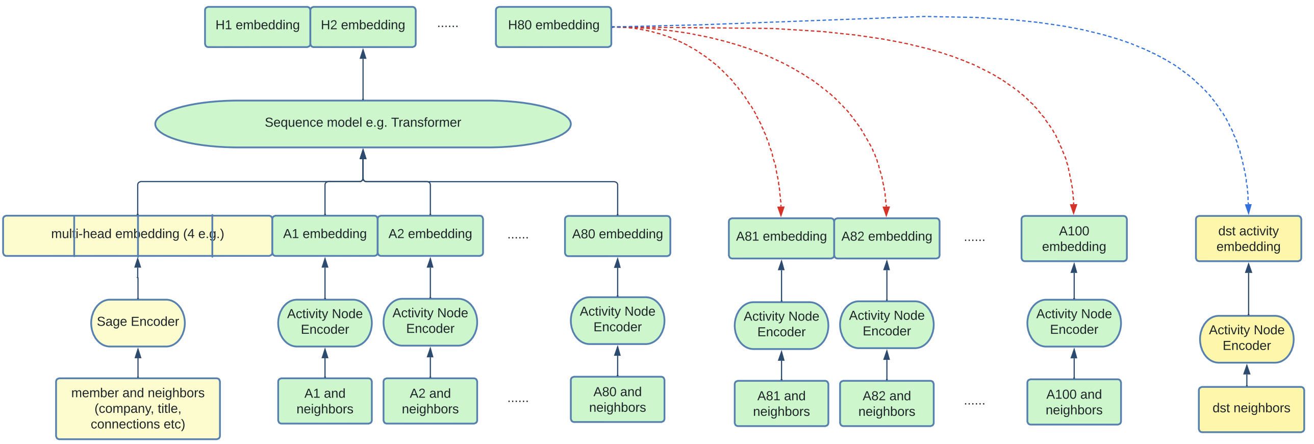 |
|---|
| Temporal GNN Framework (Figure 4 from paper) |
Graph Densification
Since GNNs rely on neighbourhood aggregation, nodes with few interactions pose a cold start problem. To solve this problem, artificial edges are added between nodes with low out-degrees and nodes with high out-degrees based on content-based similarity. Specifically, their algorithm works like so:
- Nodes with out-degree
30th percentiledesignated as low-degree - Nodes with out-degree
90th percentiledesignated as high-degree - Pre-embed all nodes with an LLM based on content
- For each low-degree node, find its approximate
top-50neighbours amongst the high-degree set. Create an edge between each of them and the low-degree node with edge weight based on embedding similarity
It seems that graph densification adds a small (0.2%-0.5%) lift to AUC both on offline and online metrics. It probably also increases the diversity of recommendations.
Personalized Page Rank Graph Sampling
Personalized Page Rank (PPR) is an adaptation of the well-known Page Rank algorithm and is widely used as a notion of node similarity. Specifically, given a source node s and a target node t, the PPR score represents the probability that a random walk originating at s will terminate at t.
In training the GNN under the GraphSAGE framework, embeddings of neighbours to a node s are aggregated together to form the representation for s. A terse way of saying the same thing is that "GNNs propagate signals across graphs". Hence, how neighbours are sampled is crucial in determining the performance of the GNN.
The simple way is Random Sampling, which simply chooses neighbours randomly amongst nodes connected to node s. This can done over a single-hop or multi-hops, and is efficient but not the most performant. The better way is PPR sampling, which chooses neighbours weighted by their PPR score, with the search space limited to nodes connected to s over k hops. This is slower but a better measure of neighbourhood.
From their experiments, 2-hop PPR sampling contributes 2.1% validation AUC lift. Adding more hops beyond 2 hops contributes marginally to performance, hence 2-hops is chosen for efficiency.
Other Tips and Tricks
The paper is full of practical tips on how to speed up training and improve stability. Here are some that stood out to me:
Adaptive Graph Sampling. IO time is correlated with number of neighbours sampled. So they start training with a small number of neighbours and increases it only when validation metric starts to stall. It seems that the final number of neighbours is capped at 200.
Mixed Precision. Mixed precision (float-16) gave roughly 10% speed up in training. But they had to be careful to retain float32 in the last layer otherwise it degraded the training process.
Data Bound. One reflection point they made is that GNN training is generally data-bound rather than compute bound. So the focus on the paper was to make data loading and processing more efficient. For example, they implemented a shared memory queue, and use the multiprocessing package to have different processes pre-fetch data from the DeepGNN Graph Engine and pre-process it simultaneously.
Wang 2024 - LLM for Pinterest Search
This paper explains Pinterest use of pre-trained LLMs to improve their search ranking model. They first fine-tune a Llama-8B model on human-labelled search relevance data, then used the model to label large amounts of unlabelled data. The unlabelled data was used to train a smaller MLP, which led to significant improvement in search performance.
Background
Pinterest curates human-labelled dataset for search relevance. For each query, a pin is classified into five ordered relevance levels:
- L5: Excellent / Highly Relevant
- L4: Good / Relevant
- L3: Complementary / Marginally Relevant
- L2: Poor / Irrelevant
- L1: Highly Irrelevant
Teacher Model
The teacher model takes the form of a standard cross encoder setup. The teacher model is either a BERT-based LLM or a decoder-style LLM. The text inputted to the LLM is of the following format:
[CLS] Query [SEP] Pin Text
The embedding of the [CLS] token is taken for BERT-based models, whilst the embedding of the final non-padding token is taken for decoder-based models (such as Llama). The embedding is passed through several fully-connected layers, and the final output dimension corresponds to the 5 relevance levels. The LLMs are fine-tuned during training by minimizing the pointwise multi-class cross entropy loss.
To enhance the representation of the pin text for the teacher model, several features are concatenated together:
- Pin titles and descriptions are used as-is
- Synthetic image captions are generated using an off-the-shelf model called BLIP
- High-engagement query tokens. Queries resulting in high engagement with a pin are aggregated over the past 2 years, and the top tokens are selected.
- User-curated Board Titles. Users curate their pins onto boards. The board titles are aggregated across users and top tokens are selected.
- Link Titles and Descriptions. A long click is defined as when a user clicks into a link to the webpage of a pin and stays
10 secondsthere. The incoming link url and description contains useful text which is mined.
A few off-the-shelf LLMs are tested as teacher models and the results reported below.
Student Model
The teacher model is used to label large amounts of unlabelled search impressions data. Specifically, for each row of data, the teacher model generates a softmax probability distribution over the 5-point relevance labels. The student model is then taught to mimic the predicted probability distribution using cross-entropy loss.
Note: The exact loss function for knowledge distillation is not covered in the paper. But the classical way is to perform knowledge distillation using KL-divergence loss. An implementation of the loss can be found here. The basic idea is to minimize KL-divergence between the teacher predicted probability distribution over labels and the student predicted probability distribution.
The student model is a simple feed forward network on a diverse set of features. It seems like some feature engineering is performed to optimize performance. Features include:
- Query-side embeddings. Pinterest has classifiers to categorize the query into a query interest type, shopping interest type etc. These categorical features are embedded using an embedding table. The SearchSage embedding for the query is also included.
- Pin-side embeddings. The PinSage pin embedding, SearchSage pin embedding etc. are included
- Query-pin interaction features. Standard query-pin match scores like BM25 score, % of query terms matched are also included as features
All features are presumably concatenated together, and passed into the MLP network. As mentioned above, this student network is trained using knowledge distillation from the teacher predictions above.
Results
The teacher and student model are evaluated using human-annotated search relevance dataset. The train set for the teacher model is around 280k rows of human-annotated data, and the remaining 30k rows are used for evaluation. The teacher model is then used to run inference on 30 million rows of unlabelled data, and then used to train the student model.
For the teacher model, scaling up the base model consistently produces better test performance (accuracy):
- BERT-base: 53.5%
- T5-base: 56.9%
- DeBERTaV3-base: 58.0%
- Llama3-8b: 60.2%
Note that the Llama3-8b model was trained using qLora.
The experiments also showed that:
- Scaling up the amount of teacher-inferred data was crucial for improving student model performance
- The teacher LLM was able to successfully transfer learning from a purely English human-annotated dataset to multiple other languages, thus allowing the student model to learn multi-lingual behaviour.
- The inclusion of additional text features for the teacher model above helped to improve performance significantly.
Takeaways
This is a simple paper that shows the power of using LLM models to bootstrap learning from a smaller product-specific dataset to distill an effective student model. This is a useful paradigm because in search systems, we often have vast amounts of unlabelled impressions data that we can use a teacher model to run inference on.
The paper also shows that scaling up the LLM is able to produce non-trivial increases in search relevance performance on the human-annotated dataset.
Solatorio 2024 - GISTEmbed
GISTEmbed: Guided In-sample Selection of Training Negatives for Text Embedding Fine-tuning
This paper proposes a way to learn embeddings using contrastive learning. The main idea is to use a guide model to filter out false negatives from training for better data quality and performance. GISTEmbed models are currently topping the MTEB benchmark.
Implementation
The method has an implementation in the SentenceTransformer package. We will walk through the implementation here.
Firstly, the loss is initialized with both a model to train and a guide model, both of which are SentenceTransformers.
In the forward step:
sentence_featuresis the input which is a list ofdict[str, Tensor]- The list is length
2if we have anchor, positive - The list is length
3if we have anchor, positive, negative
- The list is length
- The
sentence_featuresis passed into both themodeland theguideto get the respective embeddings- For
guide, we may need to re-tokenize it if the tokenizer of theguidediffers frommodel - This is done by using
batch_decodeand thentokenizeagain
- For
- Now we have
anchor,positiveandnegativeembeddings, each of shape(batch_size, embed_dim) - The
sim_matrixis used to compute pairwise cosine similarities:- The code is simply
torch.nn.CosineSimilarity(dim=-1)(embed1.unsqueeze(1), embed2.unsqueeze(0)) embed1becomes shape(batch_size, 1, embed_dim)and embed2 becomes shape(1, batch_size, embed_dim)- The similarity is compared at dimension
-1 - Broadcasting ensures that the comparison is done pairwise, such that the result is of shape
(batch_size, batch_size) - This is a common way to do pairwise similarity
- The code is simply
- Now we obtain the pairwise similarity matrices:
ap_sim,aa_sim,pp_sim,an_simguided_ap_sim,guided_aa_sim,guided_pp_sim,guided_an_sim
- The anchor positive similarity threshold is used to filter away potential false negatives
- This is simply the
guided_ap_sim.diagonal()which corresponds to the similarity between the anchor and positive in each row - Note that they use the guide model for determining the threshold
- This threshold is called
guided_sim
- This is simply the
mask_false_negativesis used to suppress false negatives- Using the
absolutestrategy, cases where theguided_sim_mat > guided_sim - self.marginwill be suppressed (set totorch.inf) - The idea is that negatives should not have a higher similarity than the threshold, otherwise there is a higher probability they are false negatives
- This function is applied to
ap_sim,aa_sim,pp_simandan_simto mask false negatives
- Using the
- Finally, we have
scoresscores = torch.cat([ap_sim, aa_sim, pp_sim, an_sim], dim=1) / self.temperature- This is of shape
(batch_size, 4*batch_size)
- We create
labelswhich istorch.arange(batch_size)- This is because the correct label is in the diagonal of
scoresmatrix
- This is because the correct label is in the diagonal of
- Finally the loss is computed via
torch.nn.CrossEntropyLoss()(scores, labels)- Each row is considered as a classification task where the label corresponds to the column position where the correct class is found
- The log softmax loss is then computed per row and averaged across rows
Sanjabi 2025 - 360Brew
360Brew: A Decoder-only Foundation Model for Personalized Ranking and Recommendation
360Brew is a 150B foundational LLM model used to centralize many LinkedIn models into one model.
For V1.0, 360Brew focused on replacing ranking tasks since they are less bounded by computational constraints in practice compared to retrieval.
Current Paradigm
The current paradigm relies on bloom embedding of ID based features for both members and items. These large embedding tables are supplemented with other engineered features such as item attributes. Some challenges with the current paradigm are:
- Cold start: ID based features cannot handle cold start, and thus a lot of work is done to learn good content-based representations
- Feature interactions: Previously,
Zhang 2025 - Qwen3 Embedding
Qwen3 Embedding: Advancing Text Embedding and Reranking Through Foundation Models
This short paper introduces the Qwen3 Embedding and reranker series, which are the strongest open source models currently for such tasks. The Qwen3 foundation decoder LLM serves as the backbone for fine-tuning and also is used to generate high quality synthetic training data. Note that Qwen3 is multi-lingual and are publicly available under the Apache 2.0 license, which means it can be used commercially.
Characteristics
The embedding and reranking models come in 3 sizes: 0.6B, 4B and 8B.
0.6B: 28 layers, embedding dimension of1024for the embedder4B: 36 layers, embedding dimension of2560for the embedder8B: 36 layers, embedding dimension of4096for the embedder
Since the 4B and 8B have same number of layers, presumably the 8B model has larger hidden sizes.
All the models have 32K sequence length limit, and are instruction aware, meaning that we can adjust the instruction at the start of the prompt to adjust the behaviour of the embedder or reranker. For the embedding models, there is also MRL support (Matryoshka Representation Learning), meaning that we can use custom dimensions from the embeddings.
Embedder
The text embeddings are obtained by appending an [EOS] token at the end of every input sequence. The final embedding is derived from the hidden state of the last layer corresponding to this [EOS] token.
Input format for queries or Documents is as follows:
{Instruction} {Query or Document}<span class="hl-subtle">endoftext</span>
The contrastive loss based on InfoNCE is used for training the embedder. Specifically, given a batch of training instances, the loss is defined as:
is cosine similarity function, is temperature and is the normalization factor which includes the positive pair + various negative pairs:
Comment on the above normalization factor:
- The second term is the similarity between each anchor query and hard negatives per query. Note that as it is written, only the hard negatives in the same row are used as negatives for each anchor query, but in theory we could use all negatives in the mini-batch.
- The third term is the similarity between pairs of queries. The assumption is that randomly selected queries should be unrelated to each other.
- The last term is the similarity between the positive document in each row (i.e. ) and all other documents (including hard negatives).
The and are mask factors designed to reduce impact of false negatives in the normalization factor . Specifically, given an anchor query or document and a potential negative query or document :
This means that for each row, we use the similarity score between the query and as a dynamic threshold to filter out false negatives. For any term in which has too high similarity exceeding this threshold (plus a small margin), we reject the false negative and mask it out. Note that this approach is reminiscent of triplet loss semi-hard masking or the GISTEmbed loss.
Reranker
The reranker is simpler, and training remains in the text paradigm. Specifically, the authors use the LLM chat template to incorporate instruction and frame the reranking task as a yes or no question:
<span class="hl-subtle">im_start</span>system
Judge whether the Document meets the requirements based on the Query and
the Instruct provided. Note that the answer can only be "yes" or "no".<span class="hl-subtle">im_end</span>
<span class="hl-subtle">im_start</span>user
<Instruct>: {Instruction}
<Query>: {Query}
<Document>: {Document}<span class="hl-subtle">im_end</span>
<span class="hl-subtle">im_start</span>assistant
<think>\n\n</think>\n\n
Instead of fitting a classifier head, no change is made to the architecture. The reranking score is computed as the likelihood ratio of the next token being yes or no:
The task then reduces to a supervised fine-tuning task, where the label is either yes for positives or no for negatives. The loss is simply the log probability of the correct label for each row (yes or no).
Multi-stage Training
The multi-stage training has emerged as a common practice for training text embedding models. The 3 stages used are as follows:
- Stage 1: Large scale synthetic data. The Qwen 32B model was used to synthesize training pairs of data across many tasks, such as retrieval, classification, semantic textual similarity.
- To create diversity, a document is taken from the Qwen3 training corpus, and top 5 similar documents are retrieved
- Qwen3 is presented with these documents and a user persona to generate a potential query
- Qwen3 is also instructed to vary the query type, length, difficulty and language for each query
- 150 million query - document pairs are generated this way
- Stage 2: High quality synthetic data
- The 150 million pairs in Stage 1 are filtered down to 12 million high quality pairs
- Specifically, only query - document pairs with cosine similarity greater than 0.7 are selected
- Stage 3: Model merging
- Model merging based on Spherical Linear Interpolation is used, which merges multiple model checkpoints saved during the fine tuning process.
Note that all 3 stages were used for the embedder, but stage 1 was omitted for the reranker as it did not help. The ablation studies show that all 3 stages are crucial for final performance of the 0.6B embedding model.
Chlon 2025 - LLMs are Bayesian in Expectation
LLMs are Bayesian, in Expectation, not in Realization
This paper uses information theoretic lens to analyze the effect of positional encoding on permutation qualities of LLMs and propose an algorithm to derive the optimal chain of thought length.
Summary
In context learning allows LLMs to adapt to new tasks using only a few examples at inference time. A theoretical framework for interpreting ICL is through the lens of bayesian inference (see Xie 2022 - ICL as Implicit Bayesian Inference). It proposes that transformers implicitly perform posterior updates over a latent concept variable, with the pretraining distribution encoding a prior over possible tasks.
This perspective has been challenged by Falck 2024 - Is ICL in LLMs bayesian?, which demonstrates empirically that transformer based language models systematically violate the martingale property. Specifically, for exchangeable data where the order of observations carries no information, bayesian posterior predictive distributions must satisfy:
For any permutation and bounded function . The experiments show that LLMs like GPT-3.5 consistently violate this property under input permutation.
This paper observes that while bayesian inference assumes exchangeable data, position encodings fundamentally break the symmetry. This is formalized using two complexity measures:
- Kolmogorov complexity of a sequence, which is permutation invariant for exchangeable data
- Conditional complexity given a specific ordering
It then shows that transformers with position encoding minimizes:
Where:
- denotes the uniform distribution over permutations consistent with sufficient statistics of the data
- For iid data, we can just sample uniformly over all permutations
- is the mutual information between sequences and their orderings
Note that this is a well known theorem (the kolomogorov version of Shannon's information identity) applied to this context.
Notations
- denotes a sequence of observations
- is the sufficient statistic for bernoulli sequences
- represents a permutation of elements
- denotes a transformer with parameters
- is the kolmogorv complexity of sequence
- is the binary entropy function
- denotes the number of chain of thought tokens
- denotes the target error tolerance
Huang 2025 - LLM-JEPA
This paper proposes to add a JEPA loss to regular supervised fine-tuning of LLMs. The JEPA loss tries to minimize distance between the encoding of two pairs of texts that should share the same representation (e.g. text: description of a regex, code: code representing the regex).
Premise
The next token prediction task of LLMs is not very amenable to JEPA-style training. However, there are subtasks that are well suited for JEPA - tasks involving two representations of the same reality. For example, in a "Natural Language to Regex" task, one may view the natural language instruction of lines containing the string dog two or more times and the regex .*(dog)(2,).* as two views of the same thing.
Normal SFT would just try to predict the regex code, token-by-token, from the natural language instruction (text). This paper advocates for adding a JEPA-style loss which tries to align the latent representation of the prediction given the input text with the latent representation of the code.
Method
Specifically, we can express the usual SFT objective of LLM training as:
That is, the loss is the cross entropy of the next token predicted by our LLM classifier against the tokens of the label. The SFT loss is usually the sum of log losses over the label tokens.
The LLM-JEPA objective adds an additional loss term to the usual SFT loss. The new loss aims to align the predictor representation of the input text with the encoder presentation of the code.
Some details:
- is a hyperparameter balancing the contribution of the two terms
- is the cosine similarity loss in this paper, i.e.
- Encoder. The encoding for text and code is taken as the
hidden_stateof the last token from the last layer.- To avoid two forward passes, this paper concatenates
textandcodeto do a single forward pass and extracts the relatively embeddings - The
attention_maskis carefully modified so thattextandcodenever attend to each other
- To avoid two forward passes, this paper concatenates
- Predictor. Instead of adding more layers, we insert one or more special
[PRED]tokens (ktokens) to the end of the concatenated sequence.- These tokens are only allowed to attend to the
textsegment (?) - We may view these as enabling additional non-linear computation to process the encoding of the
textinto a latent prediction of thecode - It is interesting because in theory, the model could learn to generate a good latent prediction on these
[PRED]tokens without affecting its next token prediction. So the fact that this separate task helps the NTP task is non-trivial.
- These tokens are only allowed to attend to the
- In sum, there are two forward passes during training Note: To check on this part:
- First pass: Over the input + label sequence (with
[PRED]tokens at the end of the input) with standard causal masking- Allows us to compute the usual SFT loss:
- Allows us to extract
- Second pass: Over the input + label sequence with special blocked masking
- Allows us to extract
- First pass: Over the input + label sequence (with
Finally, because of the increased computational cost, the authors considered dropout to reduce compute and also improve robustness. Specifically, we randomly choose forward passes where only is computed. They found that we can have high levels of dropout, e.g. while improving performance and reducing compute cost.
Findings
The paper spends quite a bit of time exploring the benefits of the JEPA loss. Here we summarize:
- LLM-JEPA aligns the encoding of
textandcode. Specifically, it results in a representation where is almost a linear transformation from . Without the JEPA loss, it is very clearly not the case. Using t-SNE, they also show two nice clusters with JEPA loss. - LLM-JEPA improves fine-tuning accuracy. The latent prediction task improves the NTP prediction capability of the LLM as measured by accuracy on downstream tasks. The gains are especially large on the regex synthesis task.
Hyperparameters
There are two main hyperparameters to tune, which is not ideal:
- controls the relative weight between and . The paper searches between .
- controls the number of predictor tokens (representing the computational capacity allocated to the predictor). The paper searches between
Code
Here we do a deep dive into the code repository for LLM-JEPA.
datasets/
The datasets/ folder comprises the train and test splits for different benchmarks stored in jsonl files. For example, one line of gsm8k looks like below. The aim is to produce the correct answer (exact match) given the system and user prompt.
{"messages": [
{"role": "system", "content": "Answer the math question, show steps."},
{"role": "user", "content": "James decides to bulk up. He weighs 120 kg and
gains 20% of his body weight in muscle and 1 quarter that much in fat.
How much does he weigh now?"
},
{"role": "assistant", "content": "He gains 120*.2=120*.2=24 24 kg in muscles
So he gains 24/4=24/4=6 6 kg of fat
That means he gains a total of 24+6=24+6=30 30 kg of bodyweight
So his new body weight is 120+30=120+30=150 150 kg
#### 150"}
]
}
Note that messages has three components: system, user, assistant.
finetune.py
Recall that the main idea is to add a loss that pushes the representation of the context towards the target. The main innovation in the code is using attention masking to create islands of causal attention for efficient computation of these representations.
Before we go into the forward pass, first note that n predictor tokens (i.e. <span class="hl-subtle">predictor_i</span>) tokens are appended to the end of each user message. This simple step allows the network to learn a non-linear prediction function over the user representation, which will be compared against the assistant representation.
Naive Approach
Let us start with the naive approach. In the forward step, there are normally three tensors to pass:
input_ids: the tokenized idsattention_mask: the attention mask for causal modelling and masking out padding tokenslabels: the labels which are the inputs shifted right
There are three views of the data:
- Without any suffix: this is the full conversation, which is the concatenation of the user message and the assistant message
- Suffixed by
_user: this is the user message - Suffixed by
_assistant: this is the assistant message
Each view of the data has its own set of attention mask. The labels are set to -100 for the _user and _assistant views, since these are used purely for computing the jepa loss and do not contribute to next token prediction loss.
The naive approach simply treats each view as independent. This means that for a batch size of B, it gets transformed into 3B size:
- The first
Bentries are for the full conversation - The next
Bentries are for the user view - The next
Bentries are for the assistant view
After the forward pass, the user and assistant hidden representations will be split up and used to compute the JEPA loss, and added to the NTP loss. Each hidden state for the user / assistant respectively would be (B, seq_len, hidden_dim). The last token embedding is extracted and cosine similarity taken between user and assistant to get JEPA loss.
Clearly, the naive approach creates 3x the normal forward pass than just using next token prediction. The goal is to use clever masking to use 2x forward passes instead.
Clever Approach
The goal is to align the representation for both user and assistant views, but the representation for both views cannot attend to each other, otherwise there would be data leakage.
The heart of the code lies with a 4D attention mask. First, for a given batch of inputs, it is initialized with:
mask = torch.full(
(batch_size * 2, 1, seq_length, seq_length),
-torch.inf
).to(device)
Note that:
- The batch size is doubled because the first half is used for the full conversation's causal mask, and the second half is used for the packed user + assistant mask.
- The singleton dimension is used to broadcast across attention heads
- We start with
-torch.inf, so that when added to attention logits before softmax, it will result in0attention weights (i.e. masked) - We start by masking all attention, then we will create gaps subsequently
Next, we compute the last token position for the user and assistant view respectively:
- The last token index is defined as the last real token before padding begins
- A utility function is used to walk each row (for the user and assistant view respectively) to find this last token
Next, we copy the input_ids and attention_mask from the assistant message into the user message, such that it starts immediately after the user message ends. This is so that we can do a single forward pass on both.
- After this operation,
input_ids_user[i]looks like:[user_tok_0, user_tok_1, ..., user_tok_N, asst_tok_0, asst_tok_1, ..., asst_tok_M, pad, pad, ...]
Now we punch holes into the attention mask. The exact implementation is not important to know, but an example will suffice. Suppose length_user=3 and length_assistant=2, then the mask for the concatenated sequence along the last two dimensions will look like:
u0 u1 u2 a0 a1
u0 [ 0 -inf -inf -inf -inf ]
u1 [ 0 0 -inf -inf -inf ]
u2 [ 0 0 0 -inf -inf ]
a0 [-inf -inf -inf 0 -inf ]
a1 [-inf -inf -inf 0 0 ]
We can see that this mask prevents the user and assistant tokens from attending to one another, so the single forward pass will allow us to get the user and assistant representations. After the forward pass, some indexing is done to extract the hidden states of the user and assistant representation respectively.
Penha 2025 - Joint-task Semantic ID
Semantic IDs for Joint Generative Search and Recommendation
This paper addresses the task of constructing semantic IDs that are useful for both search and recommendations. The main empirical finding is that constructing semantic IDs in a task specific way will necessarily degrade performance for the other task.
Methods
The baseline / single-task methods considered for constructing semantic IDs:
- Content-based. An off-the-shelf embedder is used to embed textual content of items. This is the approach used in DSI, TIGER. Specifically,
all-mpnet-base-v2was used on the concatenated metadata of each item. The embedding is then discretized. - Search-tuned IDs. Starting from
all-mpnet-base-v2, the model is fine-tuned on search data with in-batch random negatives (i.e.MultipleNegativesRankingLossfromsentence-transformers). The search data comprises of (search_query,relevant_item_metadata) pairs. The fine-tuned embedding is then discretized. - Recommendation-tuned IDs. The Efficient Neural Matrix Factorization (EMNF) method from TokenRec is used to create collaborative filtering based embeddings .
Multi-Task Methods
A few methods were explored for how to combine multi-task signals:
- Separate. This means that each task has its own set of item IDs. At inference time, search prompts can only output search tokens, and recommendation prompts can only output rec tokens.
- Fused Concat. Each embedding and are individually l2-normalized and concatenated together.
- Fused SVD. Each embedding is l2-normalized but we further dimension reduce the embedding with higher dimensional space using truncated SVD. The two embeddings are then element-wise added together.
- Multi-task. A bi-encoder is trained on both supervision signals:
(query, item)pairs from search data and(item_a, item_b)pairs from interaction data.
Semantic-id Learning Methods
The methods considered for learning semantic ID:
- RQ-kmeans. This is basically hierarchical k-means on the residuals at each level, implemented using FAISS residual quantizer.
- RQ-VAE. Implemented using
vector-quantize-pytorch - MiniBatchDictionaryEncoding. From
sklearnlibrary - ResidualLFQ from
vector-quantize-pytorch
Data / Metrics
A search and recommendation dataset is built from MovieLens25M:
62kmovies1.2Muser-item interactions (last item per user used for test)20queries per item generated usinggemini-2.0-flash
Recall at 30 is used as evaluation metric. google/flan-t5-base is used as the generative model to learn to output semantic IDs given the context (be it search or user history) using supervised fine-tuning.
Results
The results show that:
- Single-task based embeddings perform best in their own task, much better than any multi-task method. But they degrade performance on the other task very badly.
- Amongst the multi-task methods, the multi-task method of training a bi-encoder on both contexts works best.
- Amongst semantic ID tokenisation methods,
RQ-Kmeanswas the clear winner, far outperforming all other methods.RQ-VAEin particular showed degenerate results especially for the search case.
Question: Why did RQVAE perform so badly compared to the naive RQ-Kmeans? Did the authors handle the RQVAE correctly?
Huang 2026 - Semantic Tube Predictions
This paper is a follow-up to LLM-JEPA, trying to find another way to use representation regularization to improve LLM learning. It seems to be much more successful.
The main idea of the paper is to add a loss term to normal Next Token Prediction (NTP) cross entropy loss. The idea for the loss term is that trajectory of an LLM's final layer hidden representation through time steps (i.e. moving through the sequence of tokens) should be locally linear. By adding this constraint in the form of a loss term, they find that LLM learning becomes 16x more data efficient.
Hertel 2026 - LinkedIn Feed Seq Recommender
This documents LinkedIn journey moving their feed ranker from a DCNv2 pointwise ranking system to a sequential recommender system (up to 1,000 past impressions).
Challenges with LinkedIn scale:
- Sheer scale and skew with power users having many interactions vs rare users
- Posts get a lot of interactions initially, but persist for weeks
- Real time serving
Background
Existing model is a well tuned DCNv2 model
- Two DCNv2 towers:
- One for passive actions (click, skip, long well)
- One for active actions (like, comment, share)
- Each tower has a multi-task output which I suppose gets a loss against multiple binary signals using binary cross entropy loss
- The models are run on CPU in a Java stack
Problem with this approach is feature engineering: onerous feature engineering work is done to compute:
- numeric interaction counts
- content embeddings
- Learning ID embeddings
- History transforms
The bet is that a sequential causal transformer attending over raw interaction history can learn these patterns. The challenge is latency.
Sequential Model
The pipeline:
- Encode each historical interaction as a pair of tokens (post + action), so that we get an interleaved sequence of
2Tpositions forTpost impressions - Actions include click, like, skip etc.
- After the transformer processes the
2Tsequence, all the outputs atactionpositions are discarded - The
Toutputs atpostpositions are combined with other candidate context features and then used to produce multi-task predictions using a prediction head
The forward pass of the causal transformer decoder is like so:
This is a standard transformer block, with 3 design decisions that made a difference:
- Pre layer norm. Doing layer norm on instead of doing it after the
RescaleAndAdd(their form of residual connection) made a big difference to training stability - RoPE instead of absolute postion embeddings. RoPE was much more stable, because absolute position embeddings sees a skewed distribution of data across positions (large positions are under-trained).
- The position embeddings at large positions are unstable and cause degradation in prediction quality
- RescaleAndAdd. The normal residual connection is . They did , where is learnable.
Late Fusion
The late fusion design refers to keeping context features out of the causal transformer, and only appending it to the transformer outputs. This means that they did not add historical item features like popularity into the 2T sequence.
Head Architecture
The prediction head was ablated against 3 designs:
- Linear
- MLP
- DCNv2
- Mixture of Experts
Mixture of Experts was the best design.
In-Session Data Leakage
One subtle issue was that sequential models can learn to overfit to in-session correlated behaviours. This is because within each browsing session, if the user is in an engaged mode, the click behaviours can be highly correlated, and the model can learn this pattern.
At serving time, we do not immediately have access to in-session engagement labels (probably due to data freshness), causing a test time and train time mismatch.
The solution is simple - randomize the order of items within each session when constructing training sequences.
LLM Ranker
LinkedIn experimented with an LLM ranker where the content of each post was represented as text. The LLM ranker then predicts for each new post whether the engagement is Yes or No. This had some appealing qualities but the efficiency was terrible because token sequences of interaction history took tens of thousands of tokens.
Serving System
Some design choices:
- CPU for feature fetching, tracking, and request-specific transformations; GPU for pytorch inference server
- "High performance gRPC interface that wraps Apache Arrow buffers in protobuf messages for zero-copy conversion to PyTorch tensors"
- Shared context batching. Since this is a ranker, all
512candidates for a given member request shares the same interaction history. Instead of sending a batch of512, they append all candidates along with the historical context into one long sequence, then use custom attention masks to ensure that historical context attends to each other, but candidate items do not attend to each other.- PyTorch's SDPA fallback to a naive attention with custom masks, so they built a custom CUDA kernel that extends Flash Attention
- Fused data loading. Consolidating padding, batching and packing into a C++ data loader was 50% faster for the training step, avoiding python multiprocessing overhead.
Penha 2025 - SIDs for Search/Rec
Yan 2025 - LLM for Recsys
Recsys Keynote: Improving Recommendation Systems & Search in the Age of LLMs - Eugene Yan, Amazon
This talk covers future of recsys and how LLMs can be incorporated. 3 challenges:
- Cold start challenge of hash based item IDs
- Lack of metadata
- Task specific models duplicate engineering, increase maintenance cost and don't benefit from transfer learning
- Benefits: simplifies systems, reduces maintenance and transfer learning
- But there may be alignment tax
Kuaishou Example for semantic IDs
- Challenge: hash based item IDs don't encode item content and struggle with cold start and sparsity problem.
- Solution: Semantic IDs based on multimodal content
Kuaishou is a short video platform. The main problem they wanted to tackle is to help users discover new items faster.
Idea:
- Train standard ID-based embeddings for user and items
- Create cluster ID from concatenated content embeddings
- Text: BERT
- Video: ResNet
- Audio: VGGish
- Run k-means on
100 millionitems into around1kclusters- Each cluster gets an ID and also an embedding
- Incorporate cluster embedding in final embedding
Result:
-
+3.4% clicks -
+3.0% likes -
+3.6% cold start coverage(% of item impressions which are new items) -
+1.2% cold start velocity(% of new items that were able to hit some threshold of views) -
Example:
- trainable, multimodal, semantic IDs @ Kuaishou
- Short videos platform
- Problem: help users discover new items faster
Filtering Bad job recommendations at Indeed
Problem: poor user experience of email job recommendations and lost trust due to low quality job recommendations Solution: Lightweight classifier trained from GPT-4o annotated data to filter bad recs
Process:
- Start with evals - 250 labelled examples with confidence labels
- Started with open LLMs like Llama2, but performance was very bad
- Used GPT-4, which was very accurate but too slow and costly (22 secs)
- Used GPT-3.5, but had poor precision (0.63) on job recommendations
- Finetuned GPT-3.5 and got 0.9 precision at 1/4th of of GPT-4 cost and latency
- Distilled lightweight classifier on finetuned GPT-3.5 labels
Lightweight classifier was 0.86 auc-roc, with latency <200ms. Result was:
-18% bad recommendations- Expected lower application rates because recommending fewer items
unsubscribed rate -5%application rate +5%
Enriching exploratory search queries @ Spotify
Problem: Help users search for new items (podcasts, audiobooks) in a catalogue of known items (e.g. songs, artists)
- How to solve cold start issue for new categories?
- Exploratory search was essential to expand beyond music
Solution: Query recommendation system
Start creating queries from new items (e.g. podcast title, author etc.) and ask LLM to rewrite as natural language query
Unified Ranker for Search & Recsys @ Netflix
Joint Modeling of Search and Recommendations Via an Unified Contextual Recommender (UniCoRn)
Example of Stripe building a transformer based foundation model from sequence of transactions to identify fraud.
Problem: teams deal with complexity from bespoke models for search, similar item recs, pre-query recs
- High operational cost and missed transfer learning opportunities
Unified Contextual Ranker (UniCoRn) takes in a unified input schema and returns a prediction. Unified inputs:
- User ID
- item ID
- Search Query
- Task
Some clever tricks to reframe item to item recommendations as search, by using last item title as query.
Unified model used for search, pre-query filtering, video to video recs and more. Able to match or exceed previous task based models. Can iterate much faster with a unified model.
Unified Embeddings @ Etsy
Problem: How to help users get better results with highly specific or broad queries, on ever-changing inventory.
- Query
mother's day giftdoes not match product vocabulary - Lexical retrieval does not account for user preferences
Solution: Unified embedding and retrieval model
- Two tower architecture for user and product side
- Add a quality vector on the product side (rating, freshness, conversion rate) concatenated to the product vector
- Add a constant vector on the user side just to make dimensions match
Tandon 2025 - Gemini for YouTube
Teaching Gemini to Speak YouTube: Adapting LLMs for Video Recommendations to 2B+DAU - Devansh Tandon
In general, recommendations is going to have higher reach than search for most consumer apps.
The personalized recommendation problem is to learn f(user, context) = recs.
How to rethink the whole recommendation process in terms of gemini?
- Large Recommender Model (LRM): adapting gemini for recommendation tasks
- Start with a base gemini checkpoint, adapted for youtube recommendations
- Align LRM to different tasks using adapters
- Video retrieval (home, watch next, shorts, search, music)
- Video ranking
To train LRM, need to develop video tokens
- Each video is one token, so we can represent watch history
- And then output some sequence of video recs
SemanticID: tokenize videos to create a language for Youtube
- Creating the atomic language for youtube videos, move away from hash based tokenizing
Youtube video -> extract features like title, description, transcript, audio, vidoe frames -> embedding -> RQ-VAE to quantize embedding into semantic ID- E.g. a semantic ID would look like
A228 B204 C196 D413 E589 ...
Continued pre-training: get LRM to understand both English and the semantic ID "language":
- Synthetic data relationships:
- Link text and SID, e.g.
Prompt: Video [A228 ...] has titleand the response isCarlos Alcaraz vs Novak Djokovic - Create lots of synthetic data doing this
- Link text and SID, e.g.
- User behaviours: SID sequences of video watches
Prompt: A user has previously watched the following vidoes: [A110, ...], [F707, ...], [C94, ...], \n <mask1>Output: <mask1>: [B230, ...]
After doing this kind of training, we get an LRM that can reason across both English and Youtube Video language.
- e.g.
Prompt: Video [A185, ...] is interesting to tennis fans since it is about wimbledon. Video [J110 ...] is interesting to - Model can respond
Output: scientists since it is about AI
We can now perform generative retrieval with this new language. For example, we can just load context and history into the prompt, and get it to recommend new videos.
Prompt:
------
User: region US | 24 years female | device ANDROID | origin watch next|
Context video: channel Olympics | title WHAT a COMEBACK! Men's 400m | SemanticID_1 |
Watch history:
SID 1 Taylor Swift 100% 260.00s
SID 2 Kris Hui 40% 260.00s
Interestingly, compared to traditional recommenders which returns mostly men's sports videos (due to the last video being Men's 400m), the generative system was able to recommend women's sprint events.
In general:
- The LRM is able to learn very quickly, very data efficient
- Handles the toughest recs when user information is very limited
- But servicing costs are very large for YouTube scale, so alot of effort focused on reducing TPU serving cost
A simple trick to reduce serving cost is to do batch recommendations
- Build a simple video to recs table where given a seed video, get the LRM to output generic recommendations
- Prompt is something like
language {seed_lang} | duration {video_length} | age {video_age} | title {title} | channel {uploader} | {seed_sid} - Everyday, take
top 20Mof videos by views inlast 7days, and do batch inference - Use these batch recommendations to serve some users
Base Gemini is too large at YouTube scale, have to use smaller more efficient models to adapt for recsys.
LLM x RecSys Recipe
- Tokenize content
- Capture the content essence into an atomic, semantic token
- Adapt LLM: english <> domain language
- Adapt foundation model to reason across english & new tokens (bilingual)
- Prompt with user information
- Construct prompts with user information, activity, actions
- Train surface/task-specific models
Hameed 2025 - 360Brew
360Brew: LLM-based Personalized Ranking and Recommendation - Hamed and Maziar, LinkedIn AI
Pain points on current LinkedIn ML:
- Operational: costly low agility development lifecycle
- Quality: disjoint optimization
- Developer experience: slow to roll out changes to models one by one
Goal: build a foundational model capturing the lifetime member activity data that solves all LinkedIn matching problems
- Zero shot capability: works well out of the box for next prediction tasks
- Measure how well the model does on new products
- In-Context learning: Learning from few examples without needing to retrain
- How well does the model do on new users / items? [cold start]
- Follow instruction from developers / users
- User control via prompts
Development
Building the LLM:
- Need to convert user history into a prompt by verbalizing user information and activities
- Provide instruction on what problem we are solving
- At time of training use different styles for verbalization
Prompt looks something like:
## Instruction
You are provided a member's profile and a set of jobs, their description, and interactions that the member had with the jobs. For each past job, the member has taken one of the following actions: applied, viewed, dismissed, or did not interact. Your task is to analyze the job interaction data along with the member's profile to predict whether the member will apply, view, or dismiss a new job referred to as the "Question" job.
Note: Focus on skills, location, and years of experience more than other criteria.
## Member Profile
Current position: software engineer, current company: LinkedIn, Location: Sunnyvale, California.
## Past job interaction data
Member has applied to the following jobs: [Age: 2 days, Title: Software Engineer, Location: New York, Country: USA, Company: Meta, Description: . . . ]
Member has viewed the following jobs: [Age: 1 week, Title: Software Engineer, Location: Texas, Country: USA, Company: AMD, Description: . . . ]
## Question 1
Will the member apply to the following job: [Age: 1 day, Title: Software Engineer, Location: Seattle, Country: USA, Company: Apple, Description: . . . ]
## Question 2
Will the member apply to the following job: [Age: 5 days, Title: RF Engineer, Location: Bay Area, Country: USA, Company: Google, Description: . . . ]
So in contrast to YouTube's semantic IDs, LinkedIn encodes past interactions in textual form.
Development pipeline:
- Start with OSS model
- Continued pre-training
- Supervised Finetuning
- Alignment
- Generate Brew-XL
150Bmodel - Distill to
Brew-mini - Prune and quantize to
Brew-mini-turboat3Bparameters- Ablation studies show that it is critical to
first go BIG, then go small
- Ablation studies show that it is critical to
To make development cycle smooth, build in a lot of automation into the pipelines. Especially evaluation loop.
Three levers to improve model quality:
- More (and better data)
- Prepare data to maximize accuracy, distribution of different type of data
- Bigger model size
- Context length
- Longer context length means deeper user activity
- Increasing context length initially improves performance to a certain point (around
20-30k tokens) - Beyond that models don't generalize that well and performance degrades
Tasting
Performance of model is best for cold start users. Measure relative gain over production model:
5 maximum activities:+6%10 maximum activities:+4%100 maximum activities:+2%
Generalization to new domain. 360Brew model can generalize to out of domain tasks and surfaces and beat production models in those tasks.
- Increases team agility to roll out new features without training new model
Serving
Three levers to improve efficiency:
- Sparsification
- Smaller model
- Distillation from big model to small model done using SFT + KD loss
- Gradual distillation is more effective than direct distillation, i.e. go 8B model to 6B model to 3B model etc.
- Pruning is done layerwise, gradual pruning
- Quantization: Mix precision
- FP8 for all weights
- FP32 for language model head and logit processor. Important for recommendations, otherwise predictions collapse.
- Sparsification
- Star attention (reduce attention quadratic cost)
- Not every item needs to attend to every item
- When scoring, we can score multiple items at the same time (sounds like
500)- Need to make sure these items do not attend to each other
- Star attention (reduce attention quadratic cost)
Q&A:
- They use 50-60 tasks out of domain to measure the effectiveness of the model in the eval loop.
- Designed custom vLLM kernels to allow multi-item scoring by modifying the attention mask
Han 2025 - GRPO Example
This notebook shows how to finetune gpt-oss-20b using unsloth. The parameters used are:
max_seq_length = 768
lora_rank = 4
lora_alpha = lora_rank * 2
load_in_4bit = True
offload_embedding = True
The toy problem is to induce gpt-oss to learn how to output an optimized all python matmul procedure that only uses the standard library. Naturally, using optimized libraries like numpy will be a lot faster, but there is some room to improve from a naive implementation in pure python.
First, we generate some random matrices. Note that we need A_list and B_list which are list[list[float]] to pass to our pure python function.
import numpy as np
def generate_random_matrices(seed = 3407, n = 256):
random_state = np.random.RandomState(seed)
n, k, m = random_state.randint(1, n+1, size = 3)
A = np.random.uniform(-10, 10, size = (n, k))
B = np.random.uniform(-10, 10, size = (k, m))
return A, A.tolist(), B, B.tolist()
For example, a kernel generated by GPT-5 is:
# Kernel generated by GPT-5
def matmul(A, B):
B_transpose = list(zip(*B))
return [
[
sum(a*b for a, b in zip(row, col))
for col in B_transpose
] for row in A
]
Preventing Cheating
GRPO works using RL with a reward function. To get the desired behaviour, we have to find a reward function that disincentivises cheating. For example, the LLM might just come up with a solution that imports torch or numpy to get an optimized matmul function.
Firstly, we write a function called check_only_stdlib_imports that, given a string representing a python function (let's call it fn_string), checks if it imports anything outside of the python standard library. We omit the definition here as it is rather involved.
Secondly, given fn_string, we want to compile it into a python function and disallow the function from importing anything from the global name space. The following code does so:
def create_locked_down_function(function: str):
output_function = {}
exec(function, {}, output_function)
new_matmul = output_function["matmul"]
new_matmul = types.FunctionType(new_matmul.__code__, {})
return new_matmul
Some explanations:
exec(string: str, globals: dict, locals: dict)- This executes code in
stringand stores whatever definitions within the code intolocals - By specifying an empty
dictforglobals, we are disallowing the functions defined within to access the global namespace
- This executes code in
types.FunctionType(code, globals)- This creates a new function from compiled python bytecode
- It also redefines the global variables that the function can access as an empty dictionary
- So this function turns
fn_stringinto a python function, but disallows accessing any global variables and libraries
Benchmarking
Now we create the actual benchmarking function. There are some details here that we shall gloss over, but note that at a high level, we call Benchmarker.benchmark(mat_mul_fn, [A, B]) to get some statistics about the matrix multiplcation function we are testing.
import os, gc, time, statistics
import signal
from contextlib import contextmanager
class TimeoutError(Exception): pass
@contextmanager
def time_limit(seconds):
def _handler(signum, frame):
raise TimeoutError(f"Timed out after {seconds}s")
old = signal.signal(signal.SIGALRM, _handler)
signal.setitimer(signal.ITIMER_REAL, seconds)
try:
yield
finally:
signal.setitimer(signal.ITIMER_REAL, 0.0)
signal.signal(signal.SIGALRM, old)
class Benchmarker:
def __init__(self, trials = 3, loops = 1, timeout = 30):
self.buffer = np.zeros(2 * 1024 * 1024 * 1024, dtype = np.uint8)
self.trials = trials
self.loops = loops
assert timeout > 0 # Cannot be 0 since it won't work!
self.timeout = timeout
def thrash(self):
# Edit the buffer to wipe cache lines
self.buffer ^= 1
return int(self.buffer[::4096].sum())
def benchmark(self, function, arguments):
assert len(arguments) == self.loops
samples = []
exceptions = []
timed_out = 0
for _ in range(self.trials):
gc.collect(); gc.disable(); self.thrash()
t_start = time.perf_counter_ns()
for i in range(self.loops):
try:
with time_limit(self.timeout):
function(*arguments[i])
except TimeoutError as e:
timed_out += 1
except Exception as e:
exceptions.append(str(e))
t_end = time.perf_counter_ns()
gc.enable()
samples.append((t_end - t_start) // max(1, self.loops))
return {
"median_ns": int(statistics.median(samples)),
"mean_ns": int(statistics.fmean(samples)),
"stdev_ns": int(statistics.pstdev(samples) if len(samples) > 1 else 0),
"exceptions" : exceptions,
"timeouts" : timed_out,
}
Some other details:
- A timeout is added to raise an error if the function runs for too long
gcis handled to avoid garbage collection from messing up the trial timing- Some thrashing of a large
2GBbuffer is done to wipe out the L1, L2, L3 CPU caches to avoid the CPU from tapping on the cache to fast track the computation
Generate matmul function
Now we get gpt-oss to generate some matmul function, like so.
from transformers import TextStreamer
prompt = """
Create a new fast matrix multiplication function using only native Python code.
You are given a list of list of numbers.
Output your new function in backticks using the format below:
```python
def matmul(A, B):
return ...
```
""".strip()
text = tokenizer.apply_chat_template(
[{"role": "user", "content": prompt}],
tokenize = False,
add_generation_prompt = True,
reasoning_effort = "low",
)
_ = model.generate(
**tokenizer(text, return_tensors = "pt").to("cuda"),
temperature = 1.0,
max_new_tokens = 512,
streamer = TextStreamer(tokenizer, skip_prompt = False),
)
Which will give something like:
...
```python
def matmul(A, B):
"""
Multiply two matrices A and B where both are given as
lists of lists (rows) and are compatible for multiplication.
Returns the resulting matrix as a list of lists.
"""
# Transpose B so we can access its columns as rows.
B_T = [list(col) for col in zip(*B)] # O(n*m) time
result = []
for row in A: # for each row in A
res_row = []
for col in B_T: # for each column of B
# Compute dot product of row and column
dot = sum(a * b for a, b in zip(row, col))
res_row.append(dot)
result.append(res_row)
return result
```
...
Reward functions
Now we want to build up our reward function which assigns a reward score to each new generation from gpt-oss. The flow is:
- Extract the function from a generation text
- Use
create_locked_down_functionto turn it into python code - Use
Benchmarkerto test how fast it is - Using benchmark statistics, assign some scores
First we define extract_function(generation_text: str) which simply extracts the function from a generation text by looking for the triple-backticks. Omitted for brevity.
Next we create multiple reward functions that test different aspects. For example, we have function_works which just checks that the function runs without errors. Note that the function runs on a list of completions.
def function_works(completions, **kwargs):
scores = []
for completion in completions:
score = 0
response = completion[0]["content"]
function = extract_function(response)
print(function)
if function is not None:
ok, info = check_only_stdlib_imports(function)
if function is None or "error" in info:
score = -2.0
else:
try:
new_matmul = create_locked_down_function(function)
score = 1.0
except:
score = -0.5
scores.append(score)
return scores
Another reward function checks that the function is correct. As we can see, the score is higher for more accurate functions and lower for inaccurate functions.
def correctness_check(completions, **kwargs):
scores = []
# Generate some random matrices of size less than 128
A, A_list, B, B_list = generate_random_matrices(seed = np.random.randint(10000), n = 128)
for completion in completions:
score = 0
response = completion[0]["content"]
function = extract_function(response)
if function is not None:
ok, info = check_only_stdlib_imports(function)
if function is None or "error" in info:
scores.append(0)
continue
try:
new_matmul = create_locked_down_function(function)
except:
scores.append(0)
continue
try:
pred = new_matmul(A_list.copy(), B_list.copy())
except:
# Failed!
scores.append(-2.0)
continue
true = np.matmul(A, B)
amax_error, mse_error = calculate_difference(pred, true)
# Check correctness and score!
machine_epsilon = 100*np.finfo(np.float64).eps
if amax_error >= 3: score = -3.0
elif amax_error >= 2: score = -2.5
elif amax_error >= 1: score = -2.0
elif amax_error >= 0.5: score = -1.0
elif amax_error >= 100*machine_epsilon: score = 0.0
elif amax_error >= machine_epsilon: score = 1.0
else: score = 3.0
if mse_error >= 3: score += -3.0
elif mse_error >= 2: score += -2.5
elif mse_error >= 1: score += -2.0
elif mse_error >= 0.5: score += -1.0
elif mse_error >= 100*machine_epsilon: score += 0.0
elif mse_error >= machine_epsilon: score += 1.0
else: score += 3.0
scores.append(score)
return scores
Finally we have the speed check function which rewards fast implementations.
- If the LLM implementation is faster than numpy implementation, then
positiveis used (e.g. 2x faster gives+0.02) - If the LLM implementation is slower than numply implementation, then
negativeis used (e.g. 2x slower gives-0.02)
import gc
def speed_check(completions, **kwargs):
scores = []
# Generate some random matrices of size less than 256
A, A_list, B, B_list = generate_random_matrices(seed = np.random.randint(10000), n = 256)
numpy_results = benchmarker.benchmark(np.matmul, [(A, B)])
for completion in completions:
score = 0
response = completion[0]["content"]
function = extract_function(response)
if function is not None:
ok, info = check_only_stdlib_imports(function)
if function is None or "error" in info:
scores.append(0)
continue
try:
new_matmul = create_locked_down_function(function)
except:
scores.append(0)
continue
new_results = benchmarker.benchmark(new_matmul, [(A_list.copy(), B_list.copy())])
# Get score and clip to -10, 10
negative = -(new_results["median_ns"] / numpy_results["median_ns"]) / 100
positive = +(numpy_results["median_ns"] / new_results["median_ns"]) / 100
score = negative if new_results["median_ns"] >= numpy_results["median_ns"] else positive
if score >= 10: score = 10
if score <= -10: score = -10
scores.append(score)
# Free memory to counteract OOMs
gc.collect()
torch.cuda.empty_cache()
return scores
GRPOTrainer
Finally, we can prepare our dataset and set up the GRPOTrainer.
First, we create a dataset with just the prompt. We just need the prompt because we're running this in dynamic mode, where GRPOTrainer will sample a few generations for each prompt and evaluate it using the reward functions. This represents true on-policy RL.
Note also that we use reasoning_effort="low".
from datasets import Dataset
dataset = Dataset.from_list([{"prompt" : [{"role": "user", "content": prompt.strip()}], "answer" : 0, "reasoning_effort": "low"}]*1000)
maximum_length = len(tokenizer(prompt.strip())["input_ids"])
print(maximum_length)
dataset[0]
Now we setup GRPOTrainer with configuration.
max_prompt_length = maximum_length + 1 # + 1 just in case!
max_completion_length = max_seq_length - max_prompt_length
from trl import GRPOConfig, GRPOTrainer
training_args = GRPOConfig(
temperature = 1.0,
learning_rate = 5e-5,
weight_decay = 0.01,
warmup_ratio = 0.1,
lr_scheduler_type = "linear",
optim = "adamw_8bit",
logging_steps = 1,
per_device_train_batch_size = 1,
gradient_accumulation_steps = 1, # Increase to 4 for smoother training
num_generations = 2, # Decrease if out of memory
max_prompt_length = max_prompt_length,
max_completion_length = max_completion_length,
# num_train_epochs = 1, # Set to 1 for a full training run
max_steps = 100,
save_steps = 100,
report_to = "none", # Can use Weights & Biases
output_dir = "outputs",
# For optional training + evaluation
# fp16_full_eval = True,
# per_device_eval_batch_size = 4,
# eval_accumulation_steps = 1,
# eval_strategy = "steps",
# eval_steps = 1,
)
Finally we can train the model. Note that T4 GPU might take 5 minutes for one generation which might take hours to start seeing some progress on this task.
# For optional training + evaluation
# new_dataset = dataset.train_test_split(test_size = 0.01)
trainer = GRPOTrainer(
model = model,
processing_class = tokenizer,
reward_funcs = [
function_works,
no_cheating,
correctness_check,
speed_check,
],
args = training_args,
train_dataset = dataset,
# For optional training + evaluation
# train_dataset = new_dataset["train"],
# eval_dataset = new_dataset["test"],
)
trainer.train()
After training, we can use our original prompt to see the new function that the LLM generates.
text = tokenizer.apply_chat_template(
[{"role": "user", "content": prompt}],
tokenize = False,
add_generation_prompt = True,
reasoning_effort = "low",
)
from transformers import TextStreamer
_ = model.generate(
**tokenizer(text, return_tensors = "pt").to("cuda"),
temperature = 1.0,
max_new_tokens = 1024,
streamer = TextStreamer(tokenizer, skip_prompt = False),
)
Yan 2025 - Semantic IDs
- Article: https://eugeneyan.com/writing/semantic-ids/
- Code: https://github.com/eugeneyan/semantic-ids-llm
Eugene Yan's experience of training an LLM-recommender hybrid that can recommend items using natural language.
Extend the vocab
Insert semantic ID tokens like <span class="hl-subtle">sid_0</span>, <span class="hl-subtle">sid_1</span> into the vocab. Sequences of these tokens will be used to represent the catalog. So an item may be represented like:
<span class="hl-subtle">sid_start</span><span class="hl-subtle">sid_173</span><span class="hl-subtle">sid_324</span><span class="hl-subtle">sid_764</span><span class="hl-subtle">sid_768</span><span class="hl-subtle">sid_end</span>
Data
He used video games category of Amazon Reviews 2023, because it has rich product metadata and lots of behavioural data.
- Keep only products with titles longer that
20 charsand description longer than100 chars 66kproducts737krows of interactions
Training Semantic IDs
Used RQ-VAE to train semantic IDs. Will not expound on RQ-VAE here. Eugene used:
3-levelcodebook- Each level has
256codes - This has collisions on around
10%of the66k products - Added a sequentially increasing token to each ID to ensure uniqueness
Baselines
- Train a SASRec model on semantic IDs to compare against traditional SASRec
- Use Qwen3-Embedding-0.6B to encode product metadata into embeddings
- Finetune Qwen3-8B to recommend items via semantic IDs
Data Cleaning
- Clean item descriptions using Gemini 2.5 Flash to remove HTML, reduce verbosity
- Remove promotional text, standardize formatting for titles etc.
- Augment data by extracting structured metadata like product type, platform, genre, hardware type etc.
- Build user interaction histories
Training RQ-VAE
First, we get the 1,024 embeddings using Qwen3-0.6B, then l2-normalize. The RQ VAE consists of:
- An encoder
- A codebook with 3 quantization levels
- A symmetric decoder
Some tricks:
- Use rotation trick as a replacement for the straight through estimator
- Initialize codebooks with k means clustering
- Reset unused codes
- Large batch size
Metrics for measuring quality of RQ-VAE:
loss/reconstruction: How well we can reconstruct the original item embeddings after compressing and decompressingloss/vq: Combined codebook and commitment loss across all levels.- Ensures that encoder outputs and codebook vectors stay close together
loss/total: sum ofloss/vqandloss/reconstructionloss/validation: total loss but on the held out validation set. Our deciding metric.metrics/avg_residual_norm: Leftover residuals between the quantized embedding and the original embeddingmetrics/unique_ids_proportion: % of items with unique IDS in a batch- Helps to check against codebook collapse
- We want this metric to be high
- Codebook distribution
- Plot the item distribution amongst the
256codes at each level - It should look like a uniform distribution
- Plot the item distribution amongst the
Some hyperparameter tuning:
- Set :
- Tried . is the commitment weight that balances reconstruction accuracy with codebook commitment
- had the lowest validation loss, so it was chosen
- Investing in data cleaning significantly improved all the metrics
SASRec comparison
Eugene tested two SASRec variants:
- Traditional SASRec
- Each item has a unique ID with no semantic meaning
- Model uses 2 causal attention blocks, 64 dim hidden dimension, trained with binary cross entropy loss
- Dot product of embeddings is used to generate scores
- Semantic SASRec
- For semantic version, each item is a sequence of semantic tokens
- Hence for each position, the model needs to generate a sequence of tokens to represent an item
- Instead of binary cross entropy loss, we need to sum up the cross entropy loss at each position
- Question: does it make sense to add some weights to put more weightage on the first semantic token and decay it for subsequent positions?
- Teacher forcing is used for this training
- A larger model is used here, 4 causal attention blocks and 384 hidden dim
From this experiment, Eugene found that traditional SASRec is significantly better. But he puts this down to the difficulty of generating a sequence of tokens compared to directly generating one token. I also note that we are not using a pretrained LLM here, which means we are missing out on some pretrained capabilities that we could have tapped on.
Finetuning Qwen-8B
Now finally we train the language model to converse in semantic IDs.
First, we build the training dataset of 4.2 million conversations of various task types:
- Given a semantic ID, predict the item description
- Given item description, predict the semantic ID
- Predict the next item in the user's sequence
- Understand relationships between item categories
- Multi-hop reasoning
Each of these are formatted as a conversation with a system prompt, user prompt and assistant response. Now, we finetune the model in two phases.
In Phase 1, we focus on extending the model's vocabulary.
- We add
1,027new vocabulary items to the model's vocabulary, and resize the model's embedding matrix for them. - In this phase, we freeze all the model parameters except the input and output embedding layers, training
15%of total parameters - Train for
1,000steps with relatively high learning rate
In Phase 2, we do the full training:
- Train for 3 epochs on the full dataset
- 3% warmup, lower learning rate, 8-bit AdamW optimizer for memory efficiency
- Monitor progress with callbacks:
- Track gradient norms
- Measure hierarchical accuracy (I guess on different codebook granularities) on recommendation tasks
- Sample model outputs on fixed set of conversational inputs
Inference
Now the model is trained, we can have chat / recommendation conversations with it:
User: “Halo 3 Limited Edition -Xbox 360”, “Lost Planet: Extreme Condition - Xbox 360”, “Lost Planet: Extreme Condition Collector’s Edition -Xbox 360” rec
Model:
<span class="hl-subtle">sid_start</span><span class="hl-subtle">sid_64</span><span class="hl-subtle">sid_351</span><span class="hl-subtle">sid_733</span><span class="hl-subtle">sid_768</span><span class="hl-subtle">sid_end</span>
The model can also explain its recs:
User: I just finished “Dragon Quest Heroes II Explorer’s Edition - PlayStation 4”. Suggest another rec and explain why:
Model:
<span class="hl-subtle">sid_start</span><span class="hl-subtle">sid_139</span><span class="hl-subtle">sid_289</span><span class="hl-subtle">sid_534</span><span class="hl-subtle">sid_768</span><span class="hl-subtle">sid_end</span>If you liked Dragon Quest Heroes II, you might like Nights of Azure because both are action RPGs for the PlayStation 4 with a focus on combat and character progression. Both games offer a narrative-driven experience with a strong emphasis on combat mechanics, suggesting a shared player interest in this genre.
We can even have multi-turn conversation with the model:
User: I’m looking for games similar to Mario Kart. rec
Model:
<span class="hl-subtle">sid_start</span><span class="hl-subtle">sid_131</span><span class="hl-subtle">sid_503</span><span class="hl-subtle">sid_738</span><span class="hl-subtle">sid_768</span><span class="hl-subtle">sid_end</span>, <span class="hl-subtle">sid_start</span><span class="hl-subtle">sid_131</span><span class="hl-subtle">sid_260</span><span class="hl-subtle">sid_577</span><span class="hl-subtle">sid_768</span><span class="hl-subtle">sid_end</span>, <span class="hl-subtle">sid_start</span><span class="hl-subtle">sid_145</span><span class="hl-subtle">sid_416</span><span class="hl-subtle">sid_671</span><span class="hl-subtle">sid_768</span><span class="hl-subtle">sid_end</span>User: How about something similar but for Xbox? rec
Model:
<span class="hl-subtle">sid_start</span><span class="hl-subtle">sid_183</span><span class="hl-subtle">sid_461</span><span class="hl-subtle">sid_517</span><span class="hl-subtle">sid_768</span><span class="hl-subtle">sid_end</span>, <span class="hl-subtle">sid_start</span><span class="hl-subtle">sid_183</span><span class="hl-subtle">sid_461</span><span class="hl-subtle">sid_562</span><span class="hl-subtle">sid_768</span><span class="hl-subtle">sid_end</span>,<span class="hl-subtle">sid_start</span><span class="hl-subtle">sid_183</span><span class="hl-subtle">sid_461</span><span class="hl-subtle">sid_616</span><span class="hl-subtle">sid_768</span><span class="hl-subtle">sid_end</span>User: Suggest a name and description for the bundle.
Model: Xbox Racing Legends: Speed & Style Pack
Code
Here we deep dive into Eugene's code and how it is implemented. Most of the code is contained in the /src directory.
device_manager.py
The DeviceManager detects the device (cpu or cuda or mps) and is instantiated early in the scripts. The interesting part torch.set_float32_matmul_precision("high") performed when device is cuda. It's supposed to speed up float32 operations?
tokenize_items.py
This script tokenizes the product descriptions of video games:
- Uses
Qwen/Qwen3-Embedding-0.6B - Batch size =
32, max length =2048 - Reads the data from
data/output/Video_Games_items_updated.parquetinto polars - Looks for the
item_contextfield (already preprocessed) - Uses the following prompt which will be tokenized
Instruct: Given a product description, generate a semantic embedding that captures
its key features and characteristics.
Query: {original_item_text}
- Saves tokenized
input_idsandattention_masksand saves them in.npz(compressed numpy) format usingnp.savez_compressed
embed_items.py
Takes the tokenized file and embeds them.
- Writes embedded items into a parquet file
train_rqvae.py
Compresses an item embedding into hierarchical semantic IDs.
The RQVAEConfig defines the following parameters:
item_embedding_dim: embedding dim of our embedding modelencoder_hidden_dims:[512, 256, 128]the size of the VAE encodercodebook_embedding_dim:32Dimension of codebook vectors- Qn: this does not need to match qwen embedding dim?
codebook_quantization_levels:3levels in the codebookcodebook_size:256number of codes per levelcommitment_weight:0.25Commitment loss weight (beta)use_rotation_trick:TrueUse rotation trick for better gradient flowbatch_size:32768training batch size (why so large?)gradient_accumulation_steps:1num_epochs:20000scheduler_type:cosine_with_warmupwarmup_start_lr:1e-8used for cosine_with_warmupwarmup_steps:200used for cosine_with_warmupmax_lr:3e-4maximum learning rate (start of cosine)min_lr:1e-6minimum learning rate (end of cosine)use_gradient_clipping:Truegradient_clip_norm:1.0use_kmeans_init:Trueinitializes codebook vectors using k-meansreset_unused_codes:Truereset unused codes periodically to avoid collapsesteps_per_codebook_reset:2Reset unused codebook codes every N stepscodebook_usage_threshold:1.0only reset if usage falls below this proportion (0-1)val_split:0.05steps_per_train_log:10log every N stepssteps_per_val_log:200validate and checkpoint every N steps
EmbeddingDataset is a torch dataset holding the embeddings:
- Extracts all embeddings and holds them in a
torch.tensorat init- Not worried about OOM?
QuantizationOutput
QuantizationOutput is used to hold data for one quantized item:
- Holds the local loss for one codebook layer
- Subclasses
NamedTuplewhich is more lightweight thandataclass quantized_st: Tensor- The quantized vector which is passed onto the next layer
- Has the "gradient trick" (either straight through or rotation trick) applied
- Allows backpropagation into the encoder even though we passed through the non-differentiable codebook layer
quantized: Tensor- The raw nearest neighbour vectors from the codebook
- No gradients
- Observation
quantizedandquantized_stshould be identical in values, just that one has gradients attached
indices: Tensor- These are integer indices which represent the semantic IDs
loss: Tensor- The combined loss for this specific codebook layer
loss = codebook_loss + beta * commitment_loss
codebook_loss: Tensor- Measures how well the codebook vector matches the encoder output
commitment_loss: Tensor- Measures how well the encoder output matches the codebook vectors
VectorQuantizer
The VectorQuantizer implements one layer of the codebook and is the meat of the logic for training RQVAE. It will be stacked together layer multiple times to form the codebook.
- At initialization:
- Initializes with
RQVAEConfigto hold parameters - Initialize
self.embeddingto an embedding of sizecodebook_size=256, codebook_embedding_dim=32- Uniform initialization
self.embedding.weight.data.uniform_(-1 / self.codebook_size, 1 / self.codebook_size)
- Uniform initialization
- Registers some buffers for tracking codebook usage:
self.register_buffer("usage_count", torch.zeros(self.codebook_size))self.register_buffer("update_count", torch.tensor(0))
- Initializes with
find_nearest_codes(x):- Takes an input vector
x, compares it to all vectors in the codebook, and returns the nearest one - Simply uses
torch.cdistto compute distances, thentorch.argminto get the nearest - Returns a tuple of torch tensors:
- The nearest index (i.e. codeword) to
x - The quantized embedding at the index position
- The nearest index (i.e. codeword) to
- Takes an input vector
forward(x)->QuantizationOutput:- Finds the nearest index and quantized embeddings for a batch of
x- Call
find_nearest_codesto getindicesandquantized
- Call
- Applies the gradient estimator to get
quantized_st- This will be used for gradient backprop to the encoder later
apply_gradient_estimatoreither uses the straight through or rotation method
- Compute losses:
codebook_lossis the MSE loss betweenx.detach()andquantized- We want to pull the codebook embeddings toward
x
- We want to pull the codebook embeddings toward
commitment_lossis the MSE loss betweenxandquantized.detach()- We want to pull encoder output toward codebook embeddings
loss = codebook_loss + beta * commitment_loss
- Everything is packaged into
QuantizationOutputand returned self.update_usageis also called:- Updates counts of which indices were the nearest to
x - Updates the number of training steps
- Updates counts of which indices were the nearest to
- Finds the nearest index and quantized embeddings for a batch of
- Straight through
- The straight through gradient estimator simply returns
x + (quantized - x).detach() - Essentially, the embeddings passed forward is
quantized - But the vector used for gradient backprop is
x(hence straight-through back to the encodedx) - This is a naive method but works well enough
- The straight through gradient estimator simply returns
- Rotation
- The problem with the straight through estimator is that we use
quantizedfor the forward pass but usexfor the backward pass- This can be problematic especially if
qandxare far apart
- This can be problematic especially if
- The rotation idea is to apply a rotation to
xuntil it aligns withq- Since the rotation is differentiable, we get better gradients back to
x
- Since the rotation is differentiable, we get better gradients back to
- We compute (to check later):
- Let
- is the halfway vector between
uandq
- The problem with the straight through estimator is that we use
reset_unused_codes- Look up
self.usage_countto find unused indices (used0times) - Take the current batch of encoded data, and randomly select them to become the new codebook vectors
- This makes it likely for them to be used in the next forward pass since they correspond to actual encoder outputs
- All usage counters are reset after this
- Look up
RQVAE
The RQVAE class now assembles multiple VectorQuantizer into the actual VAE to create semantic IDs.
At initialization:
self.encoder: a simple MLP that shrinks the input embedding down to the codebook dimension- In this code, we go from
1024 -> 512 -> 256 -> 128 -> 32
- In this code, we go from
self.decoder: a simple MLP that goes backward from quantized vector up to embedding dimension- In this code, the decoder dims are just the reversed of the encoder dims
- So we go from
32 -> 128 -> 256 -> 512 -> 1024
- Both encoder and decoder are wrapped in
nn.Sequential self.vq_layerscontains theVectorQuantizers- It is an
nn.ModuleListof3VectorQuantizers
- It is an
forward: the main magic of this class- First we encode input item embedding
z = self.encode(x) - Also init
residual = z - Init
quantized_out = torch.zeros_like(z)- The quantization output will be the sum of
- Now we run a for loop through the vector quantizer layers:
- First we compute the quantization output for this level (which contains the mapped ID for this level etc.)
vq_output: QuantizationOutput = vq_layer(residual)
- Then we update the residual by subtracting the nearest codebook vector
residual -= vq_output.quantized.detach()
- We accumulate the codebook vectors (with gradients) into
quantized_outquantized_out += vq_output.quantized_st- Recall that the final representation passed to the decoder is
- We also accumulate the loss for each layer
vq_loss += vq_output.loss- This is the codebook + commitment loss, reconstruction loss comes later
- First we compute the quantization output for this level (which contains the mapped ID for this level etc.)
- Finally we get the total loss
- Compute the reconstruction loss
x_recon = self.decode(quantized_out)recon_loss = F.mse_loss(x_recon, x)loss = recon_loss + vq_loss
- Compute the reconstruction loss
- First we encode input item embedding
encode_to_semantic_ids: encodes an item embeddingxto an integer tensor representing its semantic IDdecode_from_semantic_ids: decodes an integer tensorsemantic_idsby looking up the codebook, summing up the levels and passing back into thedecoderkmeans_init- Runs kmeans on one batch of embeddings to initialize the codebook vectors
- Runs kmeans to get
256centroid vectors - Copies these vectors into the codebook directly
- Process layer by layer
finetune_qwen3_8b_vocab.py
This script performs Stage 1 of the qwen fine-tuning. It focuses on extending the vocabulary to include new semantic ID tokens and trains embeddings for these new tokens.
FineTuneConfig
Dataclass containing config for the training
model_name:unsloth/Qwen3-8B- Qn: Not instruction fine tuned?
load_in_4bit: Set toFalsefor embedding trainingload_in_8bit: Set toFalsenum_proc:32enable_thinking:Falsewe don't need thinking modeextend_vocabulary:Truecodebook_levels:4codebook_size:256num_semantic_tokens:1024system_prompt: see belowmax_training_samples:32000limit for training embeddinglearning_rate:1e-3batch_size:32max_steps:1000
The system prompt is as follows:
"You are a helpful AI assistant that understands and works with semantic IDs for product recommendations. Semantic IDs are hierarchical identifiers in the format
<span class="hl-subtle">sid_start</span><span class="hl-subtle">sid_105</span><span class="hl-subtle">sid_307</span><span class="hl-subtle">sid_705</span><span class="hl-subtle">sid_769</span><span class="hl-subtle">sid_end</span>that encode product relationships and categories. /no_think"
extend_tokenizer
extend_tokenizer(model, tokenizer, config: FineTuneConfig) adds semantic ID tokens to the tokenizer using Unsloth's add_new_tokens.
- Note that the vocab size affects two places:
model.get_input_embeddings().weight: the input embeddingsmodel.get_output_embeddings().weight: the language model head which predicts the next token
- First, we make sure that the vocab size of the tokenizer matches the vocab size of both the input and output embeddings
- We need to call
model.resize_token_embeddingsto get the model embedding sizes to match thetokenizer - This is because the model embeddings are padded to be multiples of
128for CUDA optimization reasons
- We need to call
- Next, we add new tokens using
unsloth.add_new_tokens:- Special tokens of
<span class="hl-subtle">rec</span>,<span class="hl-subtle">sid_start</span>,<span class="hl-subtle">sid_end</span> - Semantic IDs of
<span class="hl-subtle">sid_0</span>to<span class="hl-subtle">sid_1023</span>
- Special tokens of
prepare_model
Prepares the model for training with some additional checks:
- Freezes gradients for all parameters
- Unfreezes only the weights for the
model.get_input_embeddings()andmodel.get_output_embeddings() - Checks the trainable parameter %
load_sid_dataset
Loads the semantic IDs training dataset:
- Checks if there are texts like
<span class="hl-subtle">sid_start</span>to make sure processing is correct - Applies chat template to the rows (but keeps as text)
There are 5 distinct categories of training data:
- SemanticID -> text:
- Input: "Product
<span class="hl-subtle">sid_start</span>...<span class="hl-subtle">sid_end</span>has title:" - Output: "Super Mario Bros"
- Variations: ID to title, description, category, features or full context
- Input: "Product
- Text -> SemanticID:
- Input: "The product Super Mario Bros has SemanticID:"
- Output: "
<span class="hl-subtle">sid_start</span>...<span class="hl-subtle">sid_end</span>" - Variations: Similar variations to above
- Sequential Recommendation:
- Input: "Based on recent purchases etc., next item:"
- Output: "
<span class="hl-subtle">sid_start</span>...<span class="hl-subtle">sid_end</span>" - Variations: Various sequence lengths of 2, 3, or 5 items.
- Semantic Understanding:
- Input: "Products starting with
<span class="hl-subtle">sid_start</span><span class="hl-subtle">sid_64</span> are typically: - Output: "Nintendo switch games"
- Variations: Prefix to category, prefix to examples, similar items.
- Input: "Products starting with
- Multi-hop Reasoning:
- Input: "A user who bought
<span class="hl-subtle">sid_a</span>might also buy:" - Output: "
<span class="hl-subtle">sid_b</span> - Variations: Co-purchase patterns.
- Input: "A user who bought
DataInspectionCallback
Used to inspect training data and tokenization at each training step, by simply logging them to console.
Patterns:
DataInspectionCallbacksubclassestransformers.TrainerCallbackon_train_begin(self, args, state, control, **kwargs):- Checks the first batch of
train_dataloader - Checks batch keys
- Check shape of
batch['input_ids'] - Check shape of
batch['attention_mask'] - Check tokens and decoded of first row etc.
- Checks the first batch of
on_log(self, args, state, control, logs=None, **kwargs):- Only runs if
state.global_step % args.logging_steps == 0 - Check number of SID tokens
- Decode first example and check
- Only runs if
EmbeddingMonitorCallback
This callback aims to check how our embeddings are shifting over time.
- At initialization (or
on_train_begin), we copy the state of the initial embeddings and clone detach them - At each step, we compute the mean of the absolute difference between the current embeddings and the initial or state of embeddings from the previous step
- We also compute the per level codebook vector means etc.
- These are all logged to
wandb
SemanticIDGenerationCallback
This is a qualitative check to answer the question "If I ask the model for a recommendation right now, does it use the semantic ID tokens or does it just output plain text?"
- A fixed set of test cases are used
- The test cases are
apply_chat_template, then passed into thetokenizer, thenmodel.generateandmodel.decode - The messages are checked whether successful (SemanticIDs generated) and success rate is tracked
- Actual completion examples are logged into wandb as well
train_embeddings
The main method. Essentially we are just using unsloth SFTTrainer to do the training.
First, we set up trl.SFTConfig with a lot of the configuration we previously defined.
- Note that
dataset_text_field="text" report_to="wandb"
The trainer trl.SFTTrainer is initialized with the model, tokenizer, datasets, config and callbacks.
Then, trainer.train() is called.
Note that the model and tokenizer are initialized using unsloth.FastLanguageModel to use unsloth's optimized triton kernels.
finetune_qwen3_8b_full.py
The code is structurally very similar to the vocab finetuning run. The difference is that we are doing full training, so we unfreeze all parameters. Consequently, the learning rate needs to be much lower at 2e-5.
- Load the model from stage 1, namely
models/qwen3_8b_vocab_extended/final - A lot of the script focuses on the callbacks to evaluate recommendation quality
Cherny 2025 - Vibe Coding
Boris Cherny (creator of Claude code) has a series of tweets on how he uses Claude. This should be a good point of reference.
1. Run Claudes in 5 Terminals
Tabs are numbered 1-5. Configure system notifications to know when a claude needs input. The link provided is for iterm2 on Mac but probably can do something similar for linux or WSL.
2. Run Claudes online
Concurrently to the local terminals, he has 5-10 claudes running online at https://claude.ai/code. These can be triggered either by handing off terminal sessions to the web (using &) or manually kicking off sessions in the browser.
- Question: Does claude run in its own instance when running online? Doesn't that mean the context it has is different from the local context?
3. Use Opus 4.5 w/ Thinking all the time
Basically, use the biggest and slowest model all the time. Although it runs slower, it will complete things more reliably and with things running async, the reliability wins out in the end.
4. Use a CLAUDE.md
The claude code repo has a single CLAUDE.md that is checked into git and everyone contributes to. Everytime claude fails on a task, or does something in a slightly undesirable way (think of all the nit comments), we can add a line to CLAUDE.md so that it does not do that again.
5. Use @.claude to add stuff to CLAUDE.md
Using the claude code github action /install-github-action, tagging @.claude in PR comments we can instruct claude to add stuff to CLAUDE.md. e.g. @.claude add to CLAUDE.md to always use string literals instead of enums.
6. Start sessions in plan mode
Start in plan mode shift+tab twice, and go back and forth. Once the plan is good, switch to auto accept edits and Claude usually 1-shots the task. A good plan is super important.
7. Use slash commands for frequent workflows
Commands are commonly executed workflows that live inside .claude/commands/. These can be invoked in claude chat e.g. /commit-push-pr. This command computes git status, and some other info before getting claude to summarize and create a PR. More details at https://code.claude.com/docs/en/slash-commands#bash-command-execution. The /commit-push-pr command may be viewed here
8. Use sub-agents for more involved workflows
Slash commands are for short, simple workflows. Sub agents (living in .claude/agents) are also frequent workflows but more involved. For e.g., code simplification to simplify code after claude is done working. The code simplifier agent may be viewed here
9. Use a PostToolUse hook
Use a PostToolUse hook to format code after claude is done. Basically just bun format. We can also do ruff format etc. depending on the language.
10. Configure permissions
Do not use --dangerously-skip-permissions. Instead use /permissions and add commands that we know are safe in our environment.
11. Tool Use
Use .mcp.json to specify the MCP servers we allow claude to connect to and use tools.
12. Long Running Tasks
Use --permission-mode=dontAsk or --dangerously-skip-permissions so that claude will not get stuck. Also use hooks to ask the agent to periodically verify what is going on for monitoring.
13. Invest in the Verification Loop
This is the most important step. Claude needs a way to verify its work, whether it is through some unit tests, integration tests or browser usage etc. Having a verification feedback loop will 2x or 3x the quality.
Code Analysis
Analyzing code from different repos, constructed using code stories.
Picoclaw
Concurrent Sessions
Picoclaw (sipeed/picoclaw) currently only processes one LLM message at a time. This is blocking if we want to operate on multiple sessions at a time. Here we delve into how it currently works and how we can hack it to allow concurrent sessions.
The code story is here
- Telegram reception. We start with telegram reception, which is non-blocking. Upon receiving a user telegram message, picoclaw calls
handleMessage, which:
- Fires off some UX patterns like typing indicator, "thinking" placeholder and reactions
- Then it pushed the message onto the message bus using
PublishInbound
-
Agent loop. There is a single
AgentLoopthat is a synchronous for loop. It callsConsumeInboundto consume messages from the bus and processes them. TheprocessMessagecall will block until it calls the LLM, waits for response, call tools etc. This is the main blocking bottle neck. -
SessionKey. The
BuildAgentPeerSessionKeyis the function that determines conversation isolation based on configuration
- By default, all DM messages share the same session, but this can be configured
- All group chats get their own sessions based on channel name and group id
- If we want concurrent sessions, the session key is the natural boundary to create concurrency
- Session writing. After each
runLLMIteration, the final contents are saved for each session. These writes are keyed bySessionKey, which allows two goroutines to safely runrunAgentLoopas they read and write completely independent session files.
So if we want to hack picoclaw to support concurrent sessions (e.g. one session per telegram channel), we just need to tap on the session construct and avail it to multiple telegram channels.
Intermediate Reasoning
karpathy/autoresearch
Code Stories Link: autoresearch-end-to-end
Karpathy's autoresearch is an experiment on agent-led experimentation. The idea is really simple - there are only 3 pertinent files in the repo.
program.md - A natural language instruction on the goal and structure of the experimentation loop. It reads like a brief to a graduate student:
- Look at the git state of the repo
- Hack
train.pyto test experimental ideas - Run the experiment and read the results
- If crash, try to fix a few times and then give up
- If improved, git commit and start again
- If deproved, git reset to the original state
- Final instructions:
- Timeout: each run takes 5 mins total (note: also enforced in code)
- Crash: use judgement, fix easy bugs or give up on fundamental issues
- Never stop: never ask human for input, keep going indefinitely
prepare.py - Mostly a one-off data preparation script to download and tokenize the data. Also defines some constants that are not changeable, and the evaluation function that computes bits per byte. The agent does not touch this file.
- Important constants:
TIME_BUDGET=300: 5 min timeoutEVAL_TOKENS: fixed number of tokens for validation evaluationMAX_SEQ_LEN=2048: max sequence length
- Evaluation function:
evaluate_bpb(model, tokenizer, batch_size)computes cross entropy loss and then normalizes by total bytes of validation tokens- Cross entropy loss is expressed in
natsbecauselnis used - Divide by
ln(2)to convert nats to bits - Divide by byte count of validation tokens so that the metric is agnostic to the tokenizer vocabulary size
- Intuition is that a tokenizer with larger vocab size means that each token can represent longer words, i.e. each token carries more information bits by default
- Dataloading choice:
- Interesting packing strategy to ensure that each batch of tokens have the same length to minimize padding
- This is to squeeze out as much information as possible in the limited compute window of 5 mins
train.py - The file that the agent is supposed to hack. The code is quite sophisticated, filled with various optimization tricks that Karpathy implemented in nanochat. So it is a strong baseline, implementing the entire transformer training loop from pytorch primitives.
Will not dive into details of train.py here (that would be more of a nanochat deep dive), but some design choices:
- The training loop imports the immutable
TIME_BUDGETfromprepare.py, and imposes a stop whentotal_training_time > TIME_BUDGET evaluate_bpbis called on the model and tokenizer to get finalval_bpbwhich is printed out at the end of the run
Takeaway
That is about it! What's surprising to me is also what is not in the code: there is no sophisticated harness to ensure that the agent cannot cheat. Technically, there is nothing stopping the agent from removing the time budget from train.py or hacking the evaluation function. The takeaway is that the prompt is sufficient harness, at least for this setup and using claude.
There is also too much hype about this experiment. The tweaks that the agent makes are mostly hyperparameter changes, such as tweaking various learning rates and RoPE parameters, so it can be seen as a glorified hyperparameter tuning run which is not new.
Nonetheless, we should not downplay the usefulness of Karpathy's setup:
- Design choice of
5 minon a H100 and using bits per bytes is a neat setup to force rapid interation. He also demonstrated that a simple setup as above is sufficient to get the agent to comply - Unlike standard hyperparameter tuning, where the parameter space is pre-defined and limited scope, the entire architecture (in theory) is open to hacking. This is much more open-ended and the upper bound is unlimited. We will surely find ways to improve upon this structure and find non-trivial things using autoresearch-ish approaches. For a start, I hope to do something similar to get an agent to run through some ML experiments, using the time budget as a way to conduct effective dev runs.
Experiments
Collection of my personal experiments to validate some hypotheses.
RQ-VAE Fast Decoding
Experiments on applying RQ-VAE to fast text decoding in latent space.
Main Idea
We use ideas from two papers:
- Kaiser 2018: Fast Decoding in Sequence Models using Discrete Latent Variables
- Applies the idea of representing tokens in a shorter latent space, and then doing autoregressive text translation in the latent space, then upsample back to token space
- Still uses old VQ-VAE discretization which has issues
- Lee 2022: Autoregressive Image Generation using Residual Quantization
- Better way of doing discretization, using a codebook with multiple levels instead of a flat codebook
- Some tricks of using a specialized transformer for decoding that is faster
Experiment Goal
Verify if we can achieve significant speedup by decoding in latent space without losing accuracy
- Check perplexity on held out data
- Check codebook usage
- Compare against various base models (including qwen0.6B) on standard LLM tasks
Other goals:
- Test if RQ-transformer matches standard transformer decoding for the same compute
- Test if using a pretrained decoder backbone is necessary
- Test performance - inference speed trade-off as we increase compression factor
- Test codebook vocabulary size to codebook depth tradeoff
- Test if unsloth speeds up inference significantly
- Test if we can scale to 8B models
Overall Flow
- Start with text input (e.g.
fineweb) - Encode into a latent representation that is a shorter sequence
- Run through pretrained backbone (e.g.
qwen0.6B) - Downsample using convolutions
- Run through pretrained backbone (e.g.
- Run RQ-VAE on the latent representation to discretize into latent tokens
- This is the fast decoding part
- Decode latent tokens back into original textual space
- Upsample using de-convolutions
- Run through pretrained backbone (e.g.
qwen0.6B)
Training Sequence
The trainable components are encoder, RQ-codebook, decoder for the RQ-VAE portion, and also the RQ-transformer for the latent decoding.
- Train the RQ-VAE jointly
- Freeze pretrained qwen backbone for warmup
- Then unfreeze for full training
- Train the RQ-transformer on latent sequences
Inference Sequence
At inference time, the goal is to do autoregressive text completion (like normal LLMs):
- Given input text
- Use encoder to encode into latent space
- Use RQ-transformer to auto-regressively predict full latent sequence
- Use decoder to decode back into textual space
Code Deep Dive
Here we dive into dissecting the code in detail. The code structure is:
│ model/
│ ├── rq_vae.py
│ │ └── RQVAE ─────────────┬─► TextEncoder
│ │ ├─► ResidualQuantizer
│ │ └─► TextDecoder
│ ├── encoder.py
│ ├── decoder.py
│ ├── quantizer.py
│ ├── rq_transformer.py
│ │ ├── SpatialTransformer
│ │ ├── DepthTransformer
│ │ ├── RoPEAttention
│ │ └── TransformerBlock
│ └── layers.py
│ └── SwiGLUTransformerLayer
│ train_vae.py
│ │ ├── RQVAELightningModule
│ │ └── RQVAEDataModule
│ train_transformer.py
│ ├── RQTransformerLightningModule
│ └── RQTransformerDataModule
encoder.py
Implements TextEncoder which encodes an input text into latent embeddings representation (shorter sequence). We focus on the forward pass:
- Input text sequence:
batch_size, seq_len - Encode using pretrained
qwenbackbone:batch_size, seq_len, hidden_size - Downsample into shorter latent sequence:
batch_size, compressed_len, hidden_size- Use strided convolutions to downsample the sequence length (halves length each step)
- More details below
- Linear projection into
batch_size, seq_len, latent_dim- The
latent_dimis the dimension of our RQ-VAE codebook
- The
- Refine latents using self-attention:
batch_size, seq_len, latent_dim- Do it with
SwiGLUTransformerLayerfornum_latent_layerstimes
- Do it with
- Output the latent representation
Question: How much information do we lose in the convolutional downsampling? How can we encourage the latent space to store more information?
Diving a bit more into the convolutional downsampling process:
nn.Conv1dapplies a convolutional filter which takes a weighted sum of the input values within the windowkernel_sizeis the size of the convolution window / filter. Larger value means we average more values together.strideis how many steps we move when sliding the window.stride=2approximately halves the sequence length.paddingis the number of zero-padded cells we add to each side of the input
- For an input sequence of , padding , kernel_size , and stride , the output length is:
- The way to think about the formula is that we start with the first window (hence at the end) and then count the number of strides to take
- First we add padding to pad the input size
- Subtract because we already "occupy" the first kernel width
- Add a
flooroperator to account for partial strides which we discard
- Can use the interactive convolution explorer to visualize the convolution window
decoder.py
The decoder TextDecoder is very similar to the encoder, except we go in the other direction. From a latent sequence, we upsample using de-convolutions to return to the textual space. Again we focus on the forward pass:
- Input is a sequence of compressed latents:
batch_size, compressed_len, latent_dim - Refine latents with self-attention:
batch_size, compressed_len, latent_dim - Linear projection to hidden size:
batch_size, compressed_len, hidden_size - Upsample via transposed convolutions:
batch_size, seq_len, hidden_size - Each layer 2x expands sequence length
- Process through Qwen3 backbone (one-shot, not autoregressive):
batch_size, seq_len, hidden_size - Linear projection to vocabulary logits:
batch_size, seq_len, vocab_size
quantizer.py
Now we dive into the residual quantization portion.
The Quantizer class represents one level of the codebook. It is initialized with parameters:
dim: latent dimension of codebook vectorscodebook_size: number of vectors for this level of the codebookema_decay: the rate of updating codebook vectors (analogous to1 - learning_rate)threshold_ema_dead_code: number of dead codes we allow before we re-assign these codebook vectors
We register these buffers at init:
ema_cluster_size:torch.zeros(codebook_size)- Tracks the number of times each codebook vector is used in an exponential moving average
ema_embed_sum:torch.zeros(codebook_size, dim)- Tracks the sum of encoder embeddings assigned in an exponential moving average
The quantize method assigns an input encoder embedding x to the nearest codebook vector. Note that x would represent a residual vector (depending on the level we are at in the codebook) in the RQ-VAE architecture.
- First we use
torch.cdistto find distances to all the codebook vectors - Then we use
torch.argminto get the index of the nearest codebook vector - Then we retrieve the codebook embedding corresponding to this index
- We return a tuple
(quantized, indices)
The update_codebook_ema acts like a gradient update to the codebook vectors (following Oord 2017).
one_hot: batch_size, codebook_size = F.one_hot(indices, codebook_size)- After we run
quantizewe convert the nearest neighbourindicesinto a one-hot matrix
- After we run
cluster_size = one_hot.sum(dim=0)- The one-hot matrix is summed on dimension
0to give the number of counts per cluster - Shape is
codebook_size
- The one-hot matrix is summed on dimension
embed_sum = one_hot.t() @ x- This is the sum of encoder embeddings based on assignment to clusters
- Shape is
codebook_size, latent_dim
- The exponential moving average of
cluster_sizeandembed_sumare taken and assigned toself.ema_cluster_sizeandself.ema_embed_sumrespectively- The codebook vectors are updated as
self.ema_embed_sum / self.ema_cluster_size
- The codebook vectors are updated as
- Dead code checking to avoid codebook collapse
- Codebook collapse is the case where some codebook vectors are so far away from the encoder distribution that they never get used
- We detect these codes by tracking their exponential moving average of counts
- If the average assignment falls below a certain threshold, we delete these codebook vectors and re-initialize them to an average of a few random encoder embeddings in the batch
There is also compute_perplexity, which is used to measure the distribution of codebook utilisation using perplexity
- Perplexity is defined as of a categorical distribution with categories
- We know that entropy ranges from to
- So perplexity ranges from to
- We want the perplexity to be close to , showing that codebook utilisation is close to uniform
Question:
- Is uniform codebook utilisation optimal, or is there some way to reason about the ideal distribution of codebook utilisation?
- There seems to be some reason to reduce the codebook size as we go into deeper levels, since the variance decreases and there is higher risk of modelling noise. Is there some information theoretic way to dynamically adjust the codebook size based on the amount of information gain from that codebook level?
The ResidualQuantizer class is a stack of Quantizers based on the desired number of codebook_levels.
The forward pass is where most of the logic resides:
- We receive an input tensor
xwith shapebatch_size, seq_len, latent_dim - We run a for loop through all the
codebook_levels:quantized, indices = quantizer.quantize(residual)- Run the quantizer to get the assigned codebook vector and indices
- Update the exponential moving average for the quantizer
commitment_loss = F.mse_loss(residual, quantized.detach())- Compute the commitment loss that pushes encoder output to be near codebook vectors
- Notice the stop gradient on the codebook vectors
- Compute perplexity and keep track
- Accumulate
quantizedintoquantized_out- Recall that RQ-VAE represents each token as a sum of the codebook vectors across all levels
- Hence we sum
quantizedat each level to get our final representation - The straight-through estimator is applied to
quantized_outto get gradients flowing back to the encoder
rqvae.py
This script combines the encoder, decoder and residual quantizer into one module for joint training.
The main method is forward, which does the encode -> quantize -> decode pass and then computes loss to train all its components.
-
Firstly we receive
input_idsandattention_maskwith shapebatch_size, seq_lenfrom the tokenizer -
We call
self.encodewhich does two things and returns adict:latent = self.encoder(input_ids, attention_mask)quant_out = self.quantizer(latent)- Returns:
latent: the encoder representation in latent spacequantized: the quantized representation (sum of codebook vectors for each position)indices: the latent token sequencecommitment_lossperplexities: for tracking purposedead_code_replacements: for tracking purpose
-
logits = self.decoder(quantized, seq_len)- This decodes the quantized representation back into logits for each position
- The logits represent our predictions for each token probability for each position
-
The logits are used to compute the
reconstruction_loss- The
reconstruction_lossis the cross entropy between predicted logits and actual labels - The actual labels default to
input_idsif labels are not explicitly provided
- The
-
The total loss is computed as
reconstruction_loss + commitment_loss
NLP Course
Based on lectures from Graham Neubig's Advanced NLP Class in 2024.
Lecture 1: Introduction
A general framework for NLP systems: create a function to map an input X into an output Y, where X and/or Y involved language. Tasks include:
- Language Modelling
- Translation
- Text Classification
- Language Analysis
- Image Captioning
Challenges of NLP
- Low frequency words
- Conjugation (e.g. adjectives modifying a word)
- Negation
- Metaphor, analogy
- Other languages
Topics:
- Language Modelling Fundamentals
- Training and Inference Methods
- Experimental Design and Evaluation
- Advanced Training and Architectures
- NLP Applications
- Linguistics and Multi-Linguality
Lecture 2: Word Representation and Text Classification
Subword models aim to address issue of low-frequency words. How many words are there in the English language? This is a bit of a trick question because do we consider company or companies different words? By using subwords we can greatly reduce the vocabulary size to around 60k which is used in modern tokenizers.
Another way to address this is to use character-level models. The main issue of character-level models is that our sequences become very long, so for a fixed sequence length we cover a lot less text in the same batch size. Using subwords saves compute and memory.
Byte Pair Encoding (2015) is a very simple method to create subwords. It simply incrementally combines the most frequent token pairs together, starting at the character level. e.g. starting with the sentence newest, widest, we first combine es into a token, then est, and so on.
Another way to do this is to use Unigram Models (e.g. Kudo 2018). First we use a unigram LM that generates all words in the sequence independently. We then pick a vocabulary that maximizes the log likelihood of the corpus given a fixed vocabulary size. The optimization process is using the EM algorithm.
Sentencepiece is a highly optimized library to train both these types of subword models.
Subword nuances:
- Subword models are hard to use multilingually because they will over-segment less common languages naively
- Subword segments are sometimes arbitrary (e.g. is it
es tore st)?
Pytorch vs Tensorflow / JAX
- Pytorch is more widely used
- Pytorch favour dynamic execution vs compile + execute
Training transformers typically uses a learning rate schedule. Start low, increase in the middle and decrease toward the end. Starting with a high learning rate will lead to weird models because transformers are sensitive.
Lecture 3: Language Modelling
Generative vs Discriminative models:
- Discriminative model: a model that calculates the probability of a latent trait given the data, i.e. , where is say the sentiment and is the text
- Generative model: a model that calculates the probability of the data itself i.e.
Generative models for text are called language models. We can use LMs to generate sentences. We can also use them to score sentences (e.g. when a sentence is a concatenation of a question and answer pair). Can also use LMs to correct sentences.
Auto-regressive language models compute . Question: why do we do it auto-regressively instead of computing the entire sequence at once? The problem is computational - predicting the next token has a space of , but predicting the entire sequence is in the order of where is the length of the sequence, which is currently untractable. That being said, if we can model the entire sequence, it will probably be a lot more efficient than the auto-regressive way.
The simplest language model is count-based unigram model. By making an indepenence assumption , we just ignore all the previous words and predict the probability of a word occurring.
The maximum likelihood estimation for the probability of a given token will simply be:
Detail: parametrizing in log space. Multiplication of probabilities are re-expressed as additions in log space, because otherwise, if we multiply 100 probabilities together for a sequence of 100 tokens, we will easily underflow the numeric precision.
Correspondingly, we can define the parameters .
Moving on to higher order n-gram models, the idea is to limit the context length to one-word before the token we are predicting, and then count:
e.g. P(example | this is an) = c(this is an example) / c(this is an).
Due to sparsity of data, we need to add smoothing to deal with zero counts, i.e. instead of just using tri-gram, we smooth tri-gram and bi-gram probabilities together:
e.g. .
More sophisticated smoothing techniques are studied in Goodman 1998: An Empirical Study of Smoothing Techniques for Language Modelling.
Problems:
- Cannot share strength amongst similar words, e.g.
carandbicycle - Cannot condition on context with intervening words, e.g.
Dr Jane SmithvsDr Gertrude Smith - Cannot handle long-distance dependencies, e.g.
tennisandracquetinfor tennis class he wanted to buy his own racquet
The standard toolkit for n-gram models is kenlm which is extremely fast and scalable, written in c++.
Evaluating Language Models
- Log Likelihood:
- Per-word Log Likelihood:
- Per-word Cross Entropy:
Aside: Any probabilistic distribution can also be used to compress data. The entropy measure is closely related to the number of bits needed to store the data based on our language model.
- Perplexity. Lower is better. Perplexity is the number of times we need to sample from the probability distribution until we get the answer right.
Other Desiderata of LMs
Calibration Guo 2017. Formally, we want the model probability of the answer matching the actual probability of getting it right. Typically we measure calibration by bucketing the model output probabilities and calculating expected calibration error:
where represents a sub-segment of the data which corresponds to a confidence interval from the model.
How do we calculate answer probabilities? e.g. the university is CMU and the university is Carnegie Mellon University should both be acceptable.
- One way is to use paraphrases to substitute phrases
Jiang 2021. - One way is to just ask the model to generate a confidence score, see Tian 2023 - Just ask for calibration
Another desirable characteristic is efficiency. Some metrics are:
- Memory usage (load model only, peak memory usage)
- Latency (to first token, to last token)
- Throughput
Some efficiency tips:
- On modern hardware doing 10 operations of size 1 is much slower than doing 1 operation of size 10
- CPUs are like motorcycles and GPUs are like airplanes
- Try to avoid memory moves between CPU and GPU, and if we need to move memory, do so as early as possible (as GPU operations are asynchronous).
Lecture 4: Sequence Modelling
NLP is full of sequential data, especially those containing long range dependencies. References can also be complicated, e.g. the trophy would not fit in the suitcase because it was too big. What does it refer to? These are called winograd schemas.
Types of tasks:
- Binary classification
- Multi-class classification
- Structured Prediction. e.g. predicting the parts-of-speech tag for each word in the sentence
Sequence labelling is an important category of tasks in NLP:
- e.g. Parts of speech tagging
- Lemmatization
- Morphological tagging, e.g.
PronType=prs
Span labelling:
- Named entity resolution
- Syntactic Chunking
- Entity Linking
- Semantic role labelling
We can treat span labelling as a sequence labelling task by using beginning, in and out tags.
Three major types of sequence modelling:
- Recurrence
- Convolutional
- Attentional
Recurrent neural networks essentially unroll a computational graph through "time" (where time is the position in the sequence). This results in a vanishing gradient problem, where the gradient on the last token is largest, and the gradient becomes smaller as we move backwards towards the first token. This problem is not just present in RNNs, but in general for computation graphs, if there is important information, adding direct connections from the important nodes to the loss is one way to improve performance. This is the motivation for residual or skip-connections.
LSTM is one way of solving this problem - the basic idea is to make additive connections between time steps, which does not result in vanishing. The idea is to have different "gates" that control the information flow, and use additive connections. Additive connections solves the vanishing gradient problem because it does not modify the gradient (?).
Attention score functions:
-
Original paper in Bahdanau 2015 used a multi-layer perceptron for the attention function, which is very expressive but has extra parameters
-
Bilinear in Luong 2015:
-
Dot product:
-
Scaled Dot product (Vaswani 2017):
Note that the attention mechanism in Vaswani 2017 is essentially a bilinear function + scaling, because the weight matrices are involved in obtaining the query and key vectors.
Comparing RNN, convolution and attention, for a token at position 200 to attend to token at position 1:
- RNN will take 199 steps through the computation graph
- Convolution will take 20 steps if the convolution window is 10
- Attention will take 1 step
This is an advantage of the attention representation of text. Another advantage of attention is the computation speed. For a given text of N tokens, in order to produce N-1 token predictions for the next word at each step:
- RNN will have to sequentially run
N-1steps - Attention will do it in 1 step by masking the attention matrix suitably. This makes it much faster to train attention models.
Truncated Backpropagation is one technique to reduce computation. e.g. in the context of RNN, we might forward propagate through positions 1-10 and compute the gradients. For the next positions 11-20, the hidden state from position 10 is used for forward propagation, but we do not backpropagate the gradients back to positions 1-10.
Lecture 5: Transformers
Transformers started as cross attention (Bahdanau 2014) and evolved to self-attention (Vaswani 2017). There are two main types of transformers:
-
Encoder-Decoder model, e.g. T5 or BART. Encoder-decoder models have a separate encoder and decoder module. The encoder takes the input sequence and passes it into a transformer block to return a "context" embedding. The decoder then takes in both the "context" embedding and the output sequence (e.g. the same sentence in French for translation, or the same sentence itself shifted right for self-attention) with appropriate masking and generates a probability for each position in the output sequence. Note that the encoder module has un-masked full attention over the entire input sequence, but the decoder module is masked.
The benefit of the encoder-decoder model is that we get an embedding representation of a given input sequence which can be used for downstream tasks. But it is also less flexible because we need to have a concept of the "input sequence" vs the "output sequence", which is suitable for tasks like translation but not in text generation tasks there is no clear input/output.
-
Decoder only model, e.g. GPT or LLaMa. The decoder model simply takes in the input sequence and passes it through a transformer module, resulting in a probability for each position in the input sequence. Using appropriate causal masking, we can train the network to predict the next token at each position given only information about tokens at previous positions.
The benefit of the decoder model is fewer parameters than the encoder-decoder model. It's also more suitable for text generation tasks. In the encoder decoder framework, at each time step we need to recompute the encoder representation, because the representation at earlier positions can change with the addition of a new token. In the decoder only framework, the previous cached Q, K, V values do not change due to the causal masking, so we can re-use those in decoding the next time step. We should thus expect decoder only models to be faster at decoding.
Core concepts
Multi-head attention. The intuition for having multiple attention heads is that information from different parts of the sentence can be useful to disambiguate in different ways. Typically for a given word to attend to nearby words is useful for learning syntax, but attending to further words is useful for learning semantics.
Multi-head attention basically comprises of multiple attention modules, each with their own weights . The attention outputs are computed for each head, and then concatenated together. Since the resulting matrix will have times the size on one dimension, we pass it through a final linear transformation to get the desired dimension size (as though we only used one attention head).
In practice the attention weights across all the heads are concatenated together first before the matrix multiplication to vectorize the computation. The resulting matrix is then sliced and attention computed on each head, before concatenating together again for the final matrix multiplication.
Positional Encoding. There is no notion of position in the transformer. Positional encoding simply adds an embedding at each position to the word embedding to encode this information. Note that it is added right at the beginning to the raw token embeddings.
-
Sinusoidal Encoding was the original proposal in the Vaswani 2017 paper. The position embedding is a fixed vector at each position , where the element is for even and for odd , and . Here is an index on the dimension going from and is the dimension of the embedding.
The method is rather counter-intuitive but the basic idea is that we want the dot product between two embeddings to be high when the relative position is near and decay as we move away. The intuition is covered nicely in Kazemnejad 2019 and basically we can think of each positional embedding as analogous to a binary encoding represented by bits at each dimension. Instead of a hard or , the and functions provide a smoothed version so that we get a nice relative decay.
Note that this method does allow us to extrapolate the position embedding to longer sequences that we have not seen before in training.
-
Learnable Embeddings. This was proposed in Shaw 2018, which basically just allows the embedding at each position to be a learnable vector. The problem of this approach is that it becomes impossible to extrapolate to longer sequences in inference time.
-
Rotary Positional Encodings or RoPE. This was proposed in Su 2021. The fundamental idea is that we want the dot product of embeddings to result in a function of relative position.
Specifically, we desire that for given positions , and the respective word embeddings , the dot product of the resulting embeddings may be expressed purely as a function of their relative distance , and in so doing we lose notion of the absolute position entirely.
The paper uses trigonometry and imaginary numbers to come up with a function that satisfies this property. The benefit of losing notion of absolute position entirely means that we can extrapolate to longer sequences that we have not seen before, and RoPE extrapolates better than sinusoidal embeddings. LLaMa uses RoPE embeddings.
Stability. Problem of gradient vanishing or exploding as we pass through the layers of an rnn or transformer. Layer normalization (Ba 2016) is the traditional way to deal with this issue. The intuition is that it normalizes the outputs of each attention layer to a consistent range, preventing too much variance in the scale of outputs.
Here, is the output of an attention layer of embedding dimension and sequence length , and are the element-wise mean and standard deviation respectively across the time positions, and and are learnable vectors of dimension . Hence, if has very large or small values, the normalization process standardizes the range of values. The parameters and allow the model flexibility to shift the values to a different part of the space.
A simplification of layer norm is RMSNorm (Zhang and Sennrich 2019). It removes the mean and bias terms but does not hurt performance empirically. It is used in Llama. The only learnable parameters per layer is .
Residual Connections. Add an additive connection between input (to an attention layer) and the output.
Where is the attention layer function. It prevents vanishing gradients (since we get ) and also allows to focus on learning the difference from the input. In the self-attention context, having the residual connection also prevents the need for tokens to attend to themselves, since that is provided by itself.
Post vs Pre Layer Norm (Xiong 2020). This paper found that applying LayerNorm after the attention layer (and the residual connection) broke the residual connection, because we have , which means that we are no longer guaranteed to get the input . This led to some instability in transformer training. Instead, they found it is better to apply , which led to more stable training, since the residual connection is preserved.
Activation functions.
- Vaswani used
- LLaMA uses Swish or SiLU (Hendricks and Gimpel 2016), which is Looks a lot like ReLU but avoids the zero gradient problem.
Transformers are powerful but fickle - Vaswani 2017 used Adam with learning rate increase and decrease (warm up). This is no longer that necessary after the pre-layer norm (Xiong 2020).
AdamW (Loshchilov and Hutter 2017) is now more popular. It applies weight decay for regularization to Adam and corrects the previous implementation which applied the regularization incompletely. AdamW is thus theoretically more stable than Adam.
In summary, some comparisons. The Mamba paper found that the LLaMA architecture is 10x more efficient in terms of scaling law compared to the original Vaswani.
| Vaswani | LLaMA | |
|---|---|---|
| Norm Position | Post | Pre |
| Norm Type | LayerNorm | RMSNorm |
| Non-linearity | ReLU | SiLU |
| Position-Encoding | Sinusoidal | RoPE |
Lecture 6: Decoding Strategies
What is an LLM? It is a model that defines a conditional probability distribution of a sequence given some input sequence .
The nice thing about the conditional distribution is that we get some notion of the model's confidence about the next token to generate. The problem with the conditional distribution is hallucination, since models generally assign some small but non-zero probability to incorrect tokens, even if all the pre-training data is factual. See Kalai and Kempala 2023.
Ancestral Sampling is to sample the next token based on the indicated confidence by the model. The nice thing is that the resultant generations follow exactly the distribution of the model.
The problem with ancestral sampling is the long tail problem. Most language models have around 30k tokens, and the probabilities from the long tail adds up, so that there's a somewhat good chance of sampling something really unlikely.
The obvious solution to this problem is to ignore the long tail and only sampling from the top-k most probably tokens. This is top-k sampling. This results in only tokens that the model is somewhat confident in.
Alternatively, we could only sampling from the top-p probability mass. This is called top-p or nucleus sampling. This is to account for the case where top-k sampling is not so desirable because if most of the probability mass is only on say 3 tokens, we may only want to sample from them.
Another alternative is epsilon sampling, where we only sample tokens with some minimum probability. This ensures that we only sample from tokens where the model is somewhat confident.
Another strategy is to modify the "peakiness" of the data by controlling the distribution temperature. This is done by modifying the scaling factor for the final softmax layer. This allows the user to put more weights on the top results (temperature < 1.0) for factual answers, or spread the weights out more by increasing the temperature for say story generaion.
Contrastive Decoding is a newer idea - the idea is that we use a smaller model to improve the performance of a larger model. Instead of just decoding from the larger model's distribution, we contrastively decode by choosing outputs where the expert model thinks are more likely than the smaller model. The intuition is that both the big and small model are degenerate in similar ways (e.g. keep repeating itself), but the expert has knowledge which the smaller model does not have. Hence taking the probability difference helps to eliminate the degenerate cases and produce better results.
Mode-Seeking Decoding Methods
Instead of sampling, another approach is to try to maximize the probability of generation, i.e. mode-seeking.
Greedy decoding chooses the most likely token at each step.
However, greedy decoding does not guarantee finding the most likely sequence. e.g. the is often the most likely word, but choosing the would exclude many other sentences that may be more likely. Hence Beam Search, which ensures that we don't miss a high-probability sequence "hidden" behind a lower-probability prefix. This is a form of breadth-first search, where we maintain a few options at any point in the search.
- First, we explore the top 3 next tokens at time step 1
- Next, we explore the top 3 next tokens at time step 2 from each branch, leading to 9 options
- Then, we prune down to the top 3 paths from the 9 options and repeat the process for time step 3
In practice, beam search often results in a very non-diverse set, i.e. sentences that are very similar to each other. Hence we may want to introduce diversity into the process. Diverse beam search modifies the scoring when pruning beams to avoid choosing overly similar beams. The similarity score can be as simple as word jaccard similarity between pairs. Stochastic beam search modifies the next token selection to sampling instead of using top greedy decodings.
Minimum Bayes Risk
The question is: Do we actually want the generations with the highest probability? In general, we do find that outputs with low probability tend to be worse than those with high probability. However, when we compare amongst the top outputs where probabilities are quite close, it becomes less clear. Say e.g. we performed beam search and found the top 3 sequences:
the cat sat down - 0.3
the cat ran away - 0.25
the cat sprinted off - 0.2
the cat sat down is the highest probability sequence, but the combined probability mass is higher for the idea that "the cat left the area". So the idea is that we might prefer generations that have high agreement with other sequences (high probability and low risk).
In the equation above, refers to a random sample from the model, say 100 samples. refers to our hypothesis space, supposedly the top 10 outputs. The risk function measures the similarity of each candidate against the samples. For example, a risk function could be ROUGE score, which measures the n-gram overlap between two sequences. Generally, MBR is high performance but high cost - even if G is ROUGE-1 (i.e. unigram overlap), it significantly outperforms beam search or greedy search.
Other MBR variants: output ensembling. Post-ensemble (Kobayashi 2018) compares pairwise embedding similarity between outputs acoss models and chooses outputs with highest average similarity. self-consistency (Wang 2023) prompts for an answer using chain of thought, samples multiple outputs, and extracts the answer from each sample (ignoring the explanations). The most frequently generated answer is then chosen.
Constrained Generation
Sometimes we want to impose some constraints on the outputs, e.g. we want the model to suggest some hobbies but we do not want climbing, or more properly, say we want to omit toxic texts. Options:
-
Ask the model to exclude
climbing: often does not work -
Logit Manipulation. Set the logit for the token(s) corresponding to
climbingto be 0. This often messes up because there may be many synonyms or ways to express the same thing and its impossible to enumerate them -
Sample and Discard. We set up a new discriminator model which predicts whether a sequence corresponds to the idea of
climbingor not. This is an easier task and often people will initialize the model from the original language model and train it to predict this idea from a small set of fine-tuning data.We can then get the generative model to generate a few samples and keep only samples where the predicted probability of the idea to avoid is low. Another variant of this is FUDGE (Yang and Klein 2021), where we multiply the generative probability of the next token by the discriminator probability that the new sequence will belong to the idea that we desire (e.g. formality). The chosen token will be that which maximizes the combined score.
-
RLHF. The alignment fine-tuning using RLHF may be viewed as a way to do constrained generation. An interesting paper that discusses RLHF as bayesian inference is Korbak 2022.
Instead of fine-tuning, one way is to do reward-augmented decoding (Deng and Raffel 2023). The idea is to have a reward model that modifies the generative probabilities based on rewards. (?)
Human In the Loop Decoding
Some strategies to incorporate human intervention in the generation:
- Interleaved text. Model generates some text, human continues, then back to the model etc.
- Fine-grained replacement. Human selects some part of the generated text, and twiddles some knobs (e.g. "more descriptive" etc.)
- Choosing outputs. Model generates a few options, and human chooses one.
We could also use a model in the loop. One idea is Tree of thought prompting, which is somewhat analogous to beam search. We have the model generate a few sentences at a time, with a few samples. An external model then judges and chooses the best branches to continue generation.
Practical Considerations
To increase decoding speed, one method is speculative decoding. We generally generate tokens with a small model, but when the small model is very uncertain, the small model will generate topk samples and a large model will pick the next token. This can speed up generation significantly.
There are many libraries for fast decoding, e.g. vLLM, Outlines, disco etc. General takeaway is that a lot can be done at decoding time without needing to fine-tune the original model.
Lecture 7: Prompting Strategies
Basic Prompting. Append a textual string to be beginning of the sequence and let the model complete. Some models are trained as chatbots and require a specific prompting template, e.g. GPT, but in the backend its simply formatted into a string and passed to the model. The important thing is that we need to follow the template that the model was trained on, otherwise performance could suffer.
Post-processing refers to formatting the returned output from the LLM. E.g. ChatGPT supports markdown rendering, so if you ask it to generate a table it will generate it and then render it as a markdown table. Another form of post-processing is output selection, i.e. we extract the part of the output that we are actually interested in. We could do so by extracting keywords (e.g. fantastic, terrible) for a sentiment analysis task.
An interesting phenomenon for predicting labels is that getting the model to predict positive or negative vs 1-5 labels, the former will do better. The intuition behind this is to think about the data that the model was trained on. It is likely that the model has seen many more reviews with the works positive or excellent vs numeric labels, so it might do better with those types of labels.
Few-shot prompting (Brown 2021) basically injects a few examples of the task together with the instruction. One thing to take note of is that LLMs (especially smaller ones) are sensitive to small changes in the in-context examples:
- Example ordering (Lu 2021)
- Label balance (Zhang 2022)
- Label coverage (Zhang 2022)
Effects of few-shot prompting are also sometime counter-intuitive. For example, replacing correct labels with random labels sometimes barely hurts the accuracy of the task. This suggests that the few-shot prompts are more for getting the structure of the response correct rather than learning the desired labelling logic. Sometimes, more demonstrations can also hurt accuracy (this may be due to the longer context length confusing the model).
Chain of thought prompting (Wei 2022) basically tries to get the model to explain its reasoning before making an answer. The original idea was to include reasoning steps in the few-shot prompts to get the model to do likewise, and it found that this significantly improved the accuracy of the model. One interpretation for why this works is that it provides the model with adaptive computation time to generate the correct answer. e.g. a simple question like 1+1= may be answered immediately but some complex logical question might require several steps, and the reasoning step allows the model to generate whatever it needs to get the answer right.
The next step is unsupervised chain of thought prompting (Kojima 2022), which basically found that we can get the same results by just appending let's think step by step to the prompt, without requiring the few-shot examples.
Another idea is that structuring outputs as computer programs can help (Madaan 2022). e.g. if we want the model to output a Direct Acyclic Graph, we could represent the output as a python graph class object. The reason that this works is perhaps because programs are highly structured and there is a lot of code in the pre-training data. Another useful method is to get the model to output JSON format, which it has also seen a lot of.
Another idea is to have program-aided language models (Gao 2022). This allows the LLM to call a code interpreter or calculator to compute answers. This works especially well for numeric questions.
Prompt Engineering
One thing of take note of is that the format should match that of a trained model. e.g. leaving out the space after the colon Passage:text can lead to severe performance degradation. Changing the casing to PASSAGE: text can also degrade performance.
We can also do automatic prompt generation. e.g. use another model to paraphrase our prompt and then select the best response out of the samples. Another approach is gradient-based, where we try out different prompt words and choose the best prompt words based on some kind of loss. These types of methods can result in highly non-human sequences that somehow produce the best results, but they can also be exploited to elicit harmful responses.
Another method along these lines is Prefix tuning (Li and Liang 2021), where they train an embedding prefix that is appended to the transformer weights in each layer according to the task of interest. This is akin to LORA methods which train additional weights that are appendable to the model.
One way to view prompting is to view it as a human-interpretable prior to the model, which can be easier than fine-tuning.
Lecture 8: Fine-tuning and Instruction Tuning
The general framework is that language models are pre-trained on the semi-supervised language modelling task on a very large corpus, and then fine-tuned on a downstream task. There are two paradigms for doing this:
-
Multi-task learning. The standard multi-task learning framework is to train the multiple tasks (language modelling and downstream task) simultaneously, e.g. by alternating mini batches or combining losses together.
In Dery 2021, the paper argues that learning jointly on the language modelling and end-task produces better results than if we pre-trained and then fine tuned. The intuition is that the model will be learning representations that are useful for both tasks.
Another paper from Anthropic also shows that incorporating safety training at the beginning out-performs pre-training first and then fine-tuning to incorporate safety.
-
Pre-train then fine-tune. However, because it is so expensive to perform the language modelling, usually pre-train and fine-tune is the actual paradigm that we follow.
Full fine-tuning means to simply continue training the language model on the training data that we have. This is also called supervised fine-tuning. This can be prohibitively expensive. Rajbhandari 2019 showed that training a 65B parameter with 16-bit mixed precision without any optimizations requires around 1TB of GPU memory, which is clearly not feasible.
The simplest solution is to scale-up horizontally across multiple-GPUs. DeepSpeed ZeRo (Rajbhandari 2019) is a popular framework for doing so:
- Stage 1: partitioning the optimizer state does not hurt optimization speed much. This brings down memory per device from 120GB to 31GB across 12 devices.
- Stage 2: in addition, it partitions the gradients. This brings memory further down to 16GB.
- Stage 3: in addition, it partitions the parameters. This brings memory down to 1.9GB but severely impacts computation speed.
An alternative strategy is to only fine tune a smaller set of parameters. Adapters (Houlsby 2019) is one way to do this. The idea is to add an adapter block after each attention block. The adapter block down-projects the embedding dimensionality to something small like 16, passes it through a non-linearity, then up-projects back to the original dimension. Each adapter block only uses 2 x model_dim x adapter_dim parameters.
There are generally two benefits to parameter-efficient fine-tuning methods:
- They are much more memory efficient. This is because we only need to back-propagate gradients on nodes which are on the computation path between the adapter block sto the final loss function
- They are more robust to over-fitting on the small set of fine-tuning data
An extension to Adapters is Adapter Fusion (Pfeiffer 2020). The idea is that instead of a single adapter after each attention block, we have multiple adapters, each trained on a different task. We then add an AdapterFusion block, which is basically a multi-head attention over each adapter block, so that it can learn to choose which adapters to use automatically.
LoRA (Hu 2021) is very similar conceptually to adapters, with the important difference that it does not have any non-linearity. The idea is that we express the fine-tuned weights as follows (reference: Cameron Wolfe's blog post):
The goal is to learn with a low rank adaptation, so that it is parameter-efficient. Suppose for simplicity that . We may approximate , where . We can then simply freeze and modify the forward pass to become , and fine-tune the parameters for and . can be as small as 8 or 2, leading to a very parameter-efficient fine-tuning method. is initialized with small random values, whilst is initialized as zero, ensuring that we begin the finetuning process with the model's original outputs.
The efficiency of LoRA compared to full fine-tuning is significant. For d=512, r=8, the efficiency is around 3%.
The reason LoRA has caught on is two-fold:
- It does not require modifying the original model structure - we simply modify the
state_dictof the original model by adding the - Adapters incur additional inference latency due to the additional layers. LoRA has no additional latency at all
Lecture 8: Reinforcement Learning and Human Feedback
Fall 2024 - Reinforcement Learning and Human Feedback
So far we optimize model using maximum likelihood of next token. This paradigm has some problems:
- Problem #1: Some mistakes are worse than others, and we want to penalize more egregious mistakes more
- Problem #2: The target labels in MLE can be bad (e.g. toxic internet stuff, disinformation)
- Problem #3: Exposure bias. At training time, the prefix sequence is guaranteed to be good / normal. At generation, the prefix sequence can potentially become strange.
- One example is repeating words. In normal language, when a word is repeated twice, it is more likely that the word repeats again. Hence language models learn this behaviour.
So how do we measure how "good" an output is?
- Objective assessment. Have an annotated correct answer and match against it. This approach is good for math problems or problems with objective answers.
- GSM8K (Cobbe 2021) is a famous math problem dataset
- Human evaluation.
Database Course
Based on CMU 15-445/645 Intro to Database Systems course taught by Andy Pavlo and Jignesh Patel in Fall 2023. The youtube playlist.
Lecture 1
Course about how to design and implement a database management system. Textbook: Database System Concepts by Silberschatz, Korth and Sudarshan.
Agenda:
- Database Systems Background
- Relational Model
- Relational Algebra
- Alternative Data Models
A database is an organized collection of inter-related data that models some aspect of the real world. Databases are the core component of most computer applications. e.g. an excel spreadsheet is a database. SQLite is the most popular database as it is used in every cellphone.
Flat File Strawman
Store our database as a csv file that we manage. e.g. each line corresponds to an artist, year, country etc. Problems:
- Super slow to find the artist of interest as we use a for-loop to find each
- Super slow to update or delete an artist
- Data types are not stored on the csv file, we need to know which is an integer etc.
- Concurrent writes to the file are not supported
A Database Management System (DBMS) is a software that allows applications to store and analyze information in a database. A general purpose DBMS supports the definition, creation, querying, update and administrations of databases in accordance with some data model. Usually first choice is postgres or sqlite.
A data model is a collection of concepts for describing the data in a database. A schema is a description of a particular collection of data, using a given data model. Examples of data models:
- Relational
- Key / Value
- Graph
- Document / XML / Object
- Wide-Column / Column-family
- Array / Matrix / Vectors
- Hierarchical
- Network
- Multi-Value
1 is the most common. 2-4 are considered NoSQL models (a loose term). 7-9 are obsolete.
Relational Model
Early database applications were difficult to write. Every time the database schema or layout changed, IBM would need to rewrite database programs. Ted Codd devised the relational model to address this problem. The relational model is an abstraction. The relational model defines a database abstraction based on relations to reduce maintenance overhead. Key tenets:
- Store database in simple data structures (relations)
- Physical storage left up to the DBMS implementation
- Access data through high-level language, DBMS figures out the best execution model
A relation is an unordered set that contain the relationship of attributes that represent entities. An n-ary relation is equivalent to a table with n columns. A tuple is a set of attributes values (also known as its domain) in the relation. The special value NULL is a member of every domain.
A relation's primary key uniquely identifies a single tuple. Some DBMSs automatically create an internal primary key if a table does not define one. Primary key is a constraint that the DBMS will enforce to ensure no duplicates exist. A foreign key specifies that an attribute from one relation maps to a tuple in another relation. E.g. If we have an artist table with the artist id, and an album table with an artist column, the artist column is a foreign key.
We can impose constraints on the database that must hold for any tuple. DBMS will then prevent any modification that could violate those constraints. Unique and foreign key constraints are the most common. e.g. CREATE ASSERTION in SQL.
Data Manipulation Languages (DML)
There are two broad methods to store and retrieve information from a database:
- Procedural: the query specifies the high level strategy to find the desired result based on sets. This uses relational algebra.
- Non-Procedural (Declarative): The query specifies only what data is wanted and not how to find it. This uses relational calculus.
Relational Algebra
Fundamental operations to retrieve and manipulate tuples in a relation. Based on set algebra (unordered lists with no duplicates). Each operator takes one or more relations as its inputs and outputs a new relation. We can thus chain operators together to create more complex operations. The operations are:
- SELECT. Choose a subset of the tuples from a relation that satisfies a selection predicate (filter). Predicates act as filters to retain only tuples that fulfill the qualifying requirement. We can combine multiple predicates using conjunctions / disjunctions.
- Syntax:
SELECT * from TABLE where id="a"
- PROJECTION. Generate a relation with tuples that contains only the specified attributes. E.g. re-arrange ordering, manipulate values ( etc.) and remove unwanted attributes.
- Syntax:
- Example:
SELECT b_{id} - 100
- UNION. Generate a relation that contains all tuples that appear in one or both input relations. Note that R and S must have the same schema.
- Syntax:
- Example:
(SELECT * from R) UNION (SELECT * from S)
- INTERSECTION. Generate a relation that contains only the tuples that appear in both of the input relations.
- Syntax:
- Example:
(SELECT * from R) INTERSECT (SELECT * from S)
- DIFFERENCE. Generate a relation that contains only the tuples that appear in the first and not the second of the input relations.
- Syntax:
- Example:
(SELECT * from R) EXCEPT (SELECT * from S)
- JOIN. Generate a relation that contains all tuples that are a combination of two tuples (one from each input relation) with a common value for one or more attributes.
- Syntax:
- Example:
SELECT * FROM R NATURAL JOIN S;
- Rename
- Assignment
- Duplicate Elimination
- Aggregation
- Sorting
- Division
Relational algebra defines an ordering of the high level steps of how to compute a query. E.g.
- vs . The former will do a huge join before filtering, whereas the latter filters first before joining, which is much better.
Instead of specifying the exact operations, DBMS allow us to state the high level answer we want, and the DBMS decides on the exact operations and the ordering to perform. This abstracts away the need for the user to know which operations are more efficient. Note that the relational model is independent of the query language implementation, although SQL is the de-facto standard (with many variants).
Document Data Model
A collections of record documents containing a hierarchy of named field / value pairs. A field's value can be a scalar type, array, or another document. Modern implementations use JSON. Main reason for this model is to avoid relational object impedance mismatch, i.e. relational databases store data in rows with relationships between tables, but in object oriented languages like Python data is stored in objects with nested attributes, which could result in inefficient queries when we try to map between the two. In contrast, Document Databases store data in a nested json which closely resembles the object-oriented approach, making it easier to work with. The down side is that we could end up storing a lot of duplicate data in the json objects.
- Examples: MongoDB, RavenDB, DynamoDB etc.
Vector Data Model
One-dimensional arrays used for nearest neighbour search, used for semantic search on embeddings generated by transformer models. Native integration with modern ML tools etc. At their core, these are just systems that use specialized indexes (e.g. Meta FAISS) to perform NN search quickly.
- Examples: Pinecone, Weaviate, Milvus etc.
Lecture 2: Modern SQL
1971, the first relational query language called SQUARE was created. 1972 SEQUEL (Structured English Query Language) was created. SQL was added to ANSI standard in 1986. Current standard is SQL:2023.
- SQL:2023 - property graph queries, multi-dim arrays
- SQL:2016 - JSON, polymorphic tables etc.
Relational languages:
- Data Manipulation Langauge (DML)
- Data Definition Language (DDL)
- Data Control Language (DCL)
Important:
We should try to do everything on the database, in one big query.
Example database:
- student table:
sid,login,gpaetc. - enrolled table:
sid,cid(course id),grade - course table:
cid,name
Aggregates:
AVG(col). e.g.SELECT AVG(s.gpa) FROM student as sMIN(col)MAX(col)COUNT(col). e.g.SELECT COUNT(LOGIN) as cnt FROM student WHERE login LIKE '%@cs. Equivalently,COUNT(1). Count number of rows where their login matches the pattern.
Groupby: Get average gpa by course id.
SELECT AVG(s.gpa), e.cid
FROM enrolled as e JOIN student AS s
ON e.sid = s.sid
GROUP BY e.cid
String operations.
LIKEis used for string matching.%matches any substring, including empty strings._matches any one character.- SQL-92 defines string functions.
Window functions. Perform a sliding calculation across a set of tuples that are related. Like an aggregation but tuples are not grouped into a single output tuple.
SELECT ... FUNC-NAME(...) OVER (...)
FROM TABLE_NAME
e.g. Get row number per course id.
SELECT cid, sid
ROW_NUMBER() OVER (PARTITION BY cid)
FROM enrolled
ORDER BY cid
Nested queries. Invoke a query inside of another query to compose more complex computations. These are often difficult for the DBMS to optimize. e.g. This one below is a join written as a nested query.
outer query -> SELECT name FROM student WHERE
sid IN (SELECT sid FROM enrolled) <- inner query
e.g. Get the names of students in '15-445':
SELECT name FROM student
WHERE sid IN (
SELECT sid FROM enrolled
WHERE cid = '15-445'
)
Lateral joins. LATERAL operator allows us to reference tables preceding the expression. e.g. below, the second expression can reference t1.
SELECT * FROM (SELECT 1 AS X) AS t1,
LATERAL (SELECT t1.x+1 AS y) AS t2;
Common Table Expressions. Provides a way to write auxiliary statements for use in a larger query, i.e. a temp table just for one query.
WITH cteName (col1, col2) as (
SELECT 1, 2
)
SELECT col1 + col2 FROM cteName
Demonstration of CTEs: Find student record with the highest id that is enrolled in at least one course. We use the maxId in the temporary table below.
WITH cteCourse (maxId) AS (
SELECT MAX(sid) FROM enrolled
)
SELECT name FROM student, cteSource
WHERE student.sid = cteSource.maxId
We can also use recursion with CTE. Print the sequence of numbers from 1 to 10.
WITH RECURSIVE cteSource (counter) AS (
(SELECT 1)
UNION
(SELECT counter + 1 FROM cteSource
WHERE counter < 10)
)
SELECT * FROM cteSource
Lecture 3: Database Storage 1
Class will shift gears towards how to implement a DBMS. Focus is on a single node machine first, then move to concurrency. Today's focus is on the
Focus on
Storage hierarchy. Higher rank is faster, smaller, expensive.
- CPU Registers
- CPU Caches
- DRAM (i.e. memory)
- SSD
- HDD
- Network Storage
Items 1-3 are volatile, i.e. random access, byte-addressable (we can fetch specific bytes). Items 4-6 are non-volatile, i.e. sequential access, block-addressable. For non-volatile storage, we need to fetch data one block at a time, and accessing data in one contiguous block sequentially is much faster than trying to access blocks scattered around. CPU refers to items 1 and 2, Memory refers to item 3, Disk refers to items 4-6.
Some new storage category: Fast network storage is in between HDD and SSD. Persistent Memory is between SSD and DRAM.
DBMSs need to exploit the sequential access on non-volatile memory to maximize speed of retrieval. Hence how we store data contiguously matters in the design of the DBMS.
Access times:
- 1 ns L1 Cache Ref 1 sec
- 4 ns L2 Cache Ref 4 sec
- 100 ns DRAM 100 sec
- 16,000 ns SSD 4.4 hours
- 2,000,000 ns HDD 3.3 weeks
- 50,000,000 ns Network Storage 1.5 years
System Design Goals
The overall goal is to make it appear like we have more memory than we do:
- We want to allow the DBMS to manage databases that exceed the amount of memory available.
- Reading/ writing to disk is expensive, so it must be managed carefully to avoid large stalls.
- Random access on disk is much slower, so DBMS wants to maximize sequential access.
Disk oriented DBMS
On disk, we have database files stored in pages. Each page is a block of data. When an execution engine makes a query, it loads a page into buffer pool in memory. The buffer pool returns a 64-bit pointer to the memory location where the page is located. The execution engine interprets the layout of the page, updates it. The new page is then written back into the database file on disk.
Why not use the OS?
The DBMS could potentially use memory mapping mmap to store the contents of a file (or page) in the address space of a program. The benefit is that we can tap on the OS to decide which pages to load into physical memory and when to swap pages out. The downside is that the lack of control over memory management can lead to stalling and bad performance.
How the OS works:
- Suppose we have Page 1, ..., Page 4 on disk. There's only enough space in physical memory to load 2 pages.
- The OS represents this to the program as virtual memory, where Page 1, ..., Page 4 are available
- When the program touches Page 2, the OS will load Page 2 into physical memory and return a pointer to the program
- Suppose the program now touches Page 3 and Page 4
- The OS needs to decide which page to evict from physical memory
So the problems with using mmap to handle I/O for the DBMS:
- Transaction safety. The OS can flush dirty pages to disk at any time, even mid-write. We can get corrupted data on disk.
- I/O stalls. The DBMS does not know which pages are in memory, so the OS could stall due to page faults (fetching a page not in memory).
- Error handling. Difficult to validate pages. Any access can cause a
SIGBUSthat the DBMS needs to handle. - Performance issues. The OS has its own scheduling and data structures, and can contend with the DBMS's priorities.
There are some companies that use mmap:
- RavenDB
- ElasticSearch
- QuestDB
- MongoDB (moved away from
mmap)
So DBMS almost always wants to control things itself:
- Flushing dity pages to disk in the correct order
- Specialized pre-fetching
- Buffer replacement policy
- Thread / process scheduling
Paper on this: Are you sure you want to Use MMAP in your DBMS?
For database storage, we need to deal with two problems:
- How the DBMS represents the database in files on disk
- How the DBMS manages its memory and moves data back and forth from disk
File Storage
The DBMS stores a database as one or more files on disk typically in a proprietary format. The OS doesn't know anything about the contents of these files. There are portable file formats (e.g. parquet etc.). Early systems in 1980s further used custom filesystems on raw block storage. Most newer DBMSs do not do this.
The
A
There are 3 different notions of what a page is:
- Hardware page (typically
4KB). A hardware page is the largest block of data that the storage device can guarantee failsafe writes (i.e. if it says it wrote4KB, it actually happened). - OS Page (usually
4KB, but can be much larger) - Database Page (
512Bto32KB)
Why might a larger page size be a good idea? Sequential data access. If we request a page of 16KB, it is one call to the OS and data is stored sequentially. If we request 4 pages of 4KB each, it is potentially random access. But the downside is that writing to a larger page is slower than writing to a small one.
Page Storage Architecture
How do DBMSs map page IDs to physical location? Different approaches:
- Heap file organization <- most common
- Tree file organization
- Sequential / Sorted File Organization (ISAM)
- Hashing file organization
A heap file is an unordered collection of pages with tuples that are stored in random order.
RL Course
Lecture notes based on David Silver's Reinforcement Learning course.
Textbooks:
- An Introduction to Reinforcement Learning - Sutton and Barto
- Algorithms for Reinforcement Learning, Szepesvari
Lecture 1: Introduction
Reinforcement Learning is at the centre of many disciplines such as engineering, psychology, economics, neuroscience because it deals with the science of decision making. E.g. in neuroscience, one major part is the dopamine neurotransmitter which resembles RL. Mathematics - operations research. Economics - bounded rationality.
What makes RL different from other ML paradigms?
- There is no supervisor, only a reward signal. There is no clear correct action to take, only a reward
- The feedback is delayed, not instantaneous
- Time really matters in RL (non iid data)
- Agent's actions affect the subsequent data it receives
Examples:
- Fly stunt manoeuvres in a helicopter
- Play backgammon
- Manage an investment portfolio
- Make a humanoid robot walk
Rewards. A reward is a scalar feedback signal. Indicates how well agent is doing at step . The agent's job is to maximize cumulative reward. RL is based on the reward hypothesis.
Reward Hypothesis. All goals can be described by the maximization of expected cumulative reward.
Is a scalar feedback sufficient? David's argument is that in order to pick one action, we must always be able to compare and rank two actions. Hence we must have a way of ordering actions and it boils down to a scalar score.
Examples of rewards:
- Fly stunt manoeuvres in a helicopter:
- +ve reward for following desired trajectory
- -ve reward for crashing
- Backgammon:
- +ve / -ve reward for winning / losing a game
- Manage investment portfolio
- +ve reward for each $ in bank
Sequential decision making. Goal: select actions to maximize total future reward. We have to plan ahead, because actions may have long term consequences. It may be better to sacrifice immediate reward to gain more long term reward. Greedy approach does not work in RL.
Formalism. At each step , the agent:
- Executes action
- Receives observation from environment
- Receives reward from environment
The environment:
- Receives action
- Emits observation
- Emits reward
The history is the sequence of observations, actions, rewards.
What happens next depends on the history:
- The agent selects the next action based on the history
- The environment selects observation and reward to emit
This is a very generic framework or formalism that can handle all types of real world scenarios.
State is the information used to determine what happens next. We do not want to have to load the entire history (e.g. stream of video frames) to make a decision. Formally, state is a function of the history:
The simplest example of state is to e.g. just take the observation at the last timestamp (this worked for Atari games).
The environment state is the environment's private representation. What state the environment is in. That is, the data that the environment uses to pick the next observation / reward. The environment state is not usually visible to the agent or the algorithm.
The agent state is the agent's internal representation, i.e. it is the information used by reinforcement learning algorithms. It can be any function we choose of the history: .
A more mathematical definition of state. An information state (or Markov state) contains all useful information from the history.
Definition. A state S_t is Markov if and only if
The idea may be stated as "the future is independent of the past given the present". Once the state is known, the history may be thrown away. i.e. The state is a sufficient statistic of the future. In the helicopter example, the markov state might be something like position, velocity, angle, angular velocity etc. Having known all this information, it does not matter where the helicopter was 10 minutes ago, as we already have all the information we need to make an optimal decision next.
Two trivial statements to show that there always exists a markov state:
- The environment state is Markov by definition
- The history is Markov, albeit not a useful one
Fully observable environments. Full observability means that agent directly observes the environment state. The nice case.
Formally, this is a markov decision process (MDP).
Partially observable environments. Partial observability means that agent indirectly observes the environment. e.g.
- Robot with camera doesn't know its absolute location
- A trading agent only observes current prices
- A poker playing agent only observes public cards, not hidden cards
Now, agent state is not the same as the environment state. Formally this is a partially observable markov decision process. So now we need the agent to construct its own state representation , e.g.:
- Remember the complete history
- Build beliefs of the environment state, i.e. . So we have a probability distribution over possible states that we believe the environment is in.
- Recurrent neural network, i.e. . Use a linear transformation to combine the current observation with previous time step to get current time step.
Inside an RL agent
An RL agent may include these components:
- Policy: the agent's behaviour function
- Value function: how good is each state or action
- Model: the agent's representation of the environment
Policy. A policy is the agent's behaviour. It is a map from state to action, e.g.
- Deterministic policy,
- Stochastic policy,
Value function is a prediction of future reward, or the expected future reward. It is used to evaluate the goodness or badness of states.
Note that the value function is subscripted by . This indicates that the agent's expected future reward depends on its current policy. If the policy is causing a robot to fall a lot, the expected future reward is probably low.
Model A model predicts what the environment will do next. There are usually 2 parts to the model:
- Transitions predicts the next state (dynamics of the environment)
- Rewards predicts the next immediate reward
Formally,
Note that having a model is optional, there are many model-free methods in RL.
Maze example. We have a grid maze. The rewards are per time step. The actions are N, E, S, W. The states are the agent's current location.
- An example of a deterministic policy would be to have a fixed arrow direction for the action to take in any given grid that the agent is in.
- An example of value function is to have a number in each position showing the number of steps it would take to get to the end (but negated as we lose value each time step)
A taxonomy of RL agents:
- Value based - only using a value function, the policy is implicit
- Policy based - just have a policy function, no value function
- Actor critic - have both a value function and policy function, and try to get best of both worlds
Another categorization is model free vs model approach:
- Model free means we just go straight to policy and/or value function
- No model
- Model based approach. Try to model the environment and world first, then build the policy accordingly
Learning and Planning
Two fundamental problems in sequential decision making:
- Reinforcement learning
- The environment is initially unknown
- The agent interacts with the environment
- The agent improves its policy
- Planning
- A model of the environment is known and provided to the agent
- The agent performs internal computations with the model without any external interaction
- e.g. if when playing an atari game, we gave the model access to an atari emulator. The model then knows if it takes action , the emulator will be in this state etc. The model can then plan ahead, build a search tree etc.
Exploration and Exploitation
Reinforcement learning is like trial and error learning. But it is possible to miss out on exploring steps that can lead to more reward.
Exploration means choosing to gives up some known reward in order to find out more information about the environment. Exploitation exploits known information to maximize reward.
Examples:
- Restaurant selection:
- Exploitation: go to your favourite restaurant
- Exploration: try a new restaurant
- Online banner advertisements
- Exploitation: show the most successful advert
- Exploration: show a different and new advert
Lecture 2: Markov Decision Processes
Lecture 2: Markov Decision Processes
Markov Decision Processes formally describe an environment for Reinforcement Learning.
- The environment is fully observable, i.e. the current state fully characterizes the process
- Almost all RL problems can be characterized as an MDP
- Even continuous things like Optimal Control
- Partially observable cases can be formulated as MDPs
- Bandits are MDPs with one state
The Markov Property is central to MDPs. "The future is independent of the past given the present."
State Transition Matrix. For a Markov state and successor state , the state transition probability is defined as:
The state transition matrix defines transition probabilities from all states to all successor states .
Each row of the transition matrix sums to .
Markov Process. A Markov Process is a memoryless random process, i.e. a sequence of of random states with the Markov Property.
Definition. A Markov Process (or Markov Chain) is a tuple , where:
(i) is a (finite) set of states
(ii) is a state transition probability matrix
(iii)
Example of a Markov Process. A student can transit from Class 1 to Class 2 to Class 3, Pass or Sleep or Pub based on transition probabilities. We can sample episodes for the markov chain. E.g. one episode may be C1 C2 C3 Pass Sleep.
The transition probability matrix may look something like the below. Note that Sleep is the terminal state, so its self-probability is 1.0.
A markov reward process is a markov chain with values.
Definition. A Markov reward process is a tuple :
- is a finite set of states
- is a transition probability matrix,
- is a reward function,
- is a discount factor,
Definition. The return is the total discounted reward from time step .
There is no expectation because is one sample run of the Markov reward process. We'll take expectation later to get the expected return over infinite runs.
- Note that the discount factor is the present value of future rewards. implies maximally short-sighted and implies maximally far-sighted.
- The value of receiving reward after time steps is
- This setup values immediate reward above future reward
Most Markov reward and decision processes are discounted. Why?
- We do not have a perfect model, so the expected future rewards are more uncertain. Hence we put higher weights on immediate rewards.
- Avoids inifite returns in cyclic Markov processes
- If the reward is financial immediate rewards earn more interest than delayed rewards
- Animal / human behaviour shows preference for immediate rewards
- It is sometimes possible to use undiscounted Markov reward processes, e.g. if all sequences terminate
The value function gives the long-term value of state .
Definition. The state value function of an MRP is the expected return stating from state :
How do we compute the state value function? One way is to sample returns from the MRP. e.g. stating from and :
C1 C2 C3 Pass Sleep:-2.25C1 FB FB C1 C2 Sleep:-3.125
Consider if we set . Then the value function , i.e. the value is just the immediate reward.
Now the important Bellman equation for MRPs:
It essentially tells us that the value function can be decomposed into two parts:
- Immediate reward
- Discounted value of successor state
- Note that in the second-to-last line, the argument inside is a random variable, to express the fact that the state at time is random.
- Note that both and are random variables, which express the value function at each possible state at time step .
- becomes due to the law of iterated expectations. Recall that . (Not very sure exactly how this works out.)
To dig into bellman equation a bit more. Use a 1-step look ahead search. We start at state , we look ahead one step and integrate over the probabilities of the next time step. Hence we get .
We can use the bellman equation to verify if our value function is correct. Taking the value at a particular state, we can check if it is indeed the sum of the immediate reward and the weighted sum of values in all possible next steps.
The Bellman equation can be expressed concisely using matrices,
The bellman equation is a linear equation and can be solved directly using matrix inversion.
The complexity due to the matrix inversion if for states, which is not feasible for a large number of states. There are many iterative methods which are more efficient:
- Dynamic programming
- Monte Carlo evaluation
- Temporal Difference learning
Markov Decision Process
So far it has been a building block. The MDP is what we really use. A Markov Decision Process (MDP) is a markov reward process with decisions (actions). It is an environment in which all states are Markov.
Definition. A Markov Decision Process is a tuple
- is a finite set of states
- is a finite set of actions
- is a transition probability matrix with
- is a reward function,
- is a discount factor
Note that the transition probabilities and reward functions now also depend on an action, in which we can have some agency now. We can choose actions to influence the reward and values.
Definition. A policy is a distribution over actions given states,
A policy fully defines the behaviour of an agent. Some properties of a policy:
- It only depends on the current state (not the history)
- The policy does not depend on the time step (i.e. stationary)
We can still obtain the optimal policy because of the markov property - the current state captures all relevant information to make the optimal decision.
Definition. The state-value function of an MDP is the expected return starting from state , and following policy :
Definition. The action-value function of an MDP is the expected return starting from state , taking action , and following policy :
Bellman Expectation Equation. The state-value function can again be decomposed into immediate reward plus discounted value of the successor state.
Similarly we can do so for the action-value function, by inserting the chosen action:
From a given state, we have a value function attached to that state, i.e. . From this state, we have some possible actions to take. The policy determines the probability distribution over which action to take. With each action comes an action-value function . Hence we have:
Another way to look at it. We start with having chosen a particular action. Having chose a particular action, the environment will determine the particular state I end up in (based on the transition probability matrix ). Hence we have:
Now we can stitch these two perspectives together. Starting from a particular state, we can write in terms of , then write in terms of again. This will allow us to get a recursive relationship of in terms of and allow us to solve the equation.
The bellman expectation equation for is thus:
The math is expressing a simple idea: that the value at a particular state is the weighted sum of values from all possible actions we take under the current policy . The value of each action is in turn affected by the reward function and the transition probability that determines the state we end up in after taking a particular action.
Similarly, we can do the same by starting at an action instead of a state. The bellman expectation equation for is thus:
Optimal Value Function
So far we have been defining the dynamic process of the MDP, but have not tried solving the optimization problem. We will turn to this now.
Definition. The optimal state-value function is the maximum value function over all policies: The optimal action-value function is the maximum action-value function over all policies:
The MDP problem is solved once we find . We thus need some algorithms to systematically find .
Define a partial ordering over policies:
Theorem. For any MArkov Decision Process:
- There exists an optimal policy that is better than or equal to all other policies, i.e.
- All optimal policies achieve the optimal value function, i.e.
- All optimal policies achieve the optimal action-value function, i.e.
How do we find the optimal policy? An optimal policy can be found trivially by maximizing over , if we knew it. That is, we always pick the action with the highest value. Hence if we have , we have .
Intuitively, we find the optimal policy by starting at the end (resting), and iteratively look backward. This is the same kind of intuition for the Bellman optimality equations.
The optimal value of being in a state is the highest value action we can take in that state. Note that we use instead of a generic because we are choosing from the optimal action-value function.
The optimal value of an action is the weighted sum of values of states that we can end up in after taking the action. Note that in this step, we do not get to choose an action - the transition probabilities will determine what state we end up in after taking actions :
Finally, stitching these two equations together, we get the bellman optimality equation for :
How do we solve the bellman optimality equations? It is now non-linear due to the max function, so we cannot solve it with matrix inversion as before. There is no closed form solution in general, but there are many iterative solution methods:
- Value iteration
- Policy iteration
- Q-learning
- Sarsa
Intuition. The core idea behind the bellman equations is to break down a complex sequential decision problem into a series of simpler, recursive steps. Imagine we are at a particular point in time and in a particular state. The bellman equations tell us that if we can assume that we will act optimally for all future steps after this action, then the problem of finding the best current action becomes trivial - we simply choose the action that yields the highest expected value (based on assuming future optimality).
To actually start unravelling the equations and solving them, we start from the termination point of a process (where the assumption of future optimality trivially holds) and work backwards.
Lecture 3: Planning by Dynamic Programming
Lecture 3: Planning by Dynamic Programming
What is dynamic programming?
- Dynamic: sequential or temporal component to the problem
- Programming: optimising a mathematical "program", i.e. a policy
It is a method for solving complex problems, by breaking them into subproblems that are simpler to solve.
Dynamic Programming is a very general solution method for problems which have two properties:
- Optimal substructure: the pricniple of optimality applies. The optimal solution can be decomposed into subproblems.
- e.g. to find the shortest path from A to B, we can find the shortest path from A to midpoint, and then find the shortest path from midpoint to B, and then combine the paths together.
- Overlapping subproblems. The subproblems need to recur many times and solutions can be re-used.
- e.g. if we have the shortest path from midpoint to B, we can reuse that to find the shortest path from C to B if it traverses the midpoint as well.
Note that Markov Decision Processes satisfy both properties:
- The bellman equations decompose the large problem into recursive steps
- The value functions for a particular state cache the sub-solutions and are re-used
Planning by dynamic programming. Planning is a different problem from RL. Someone tells us the dynamics of the MDP, and we try to solve it.
- Assume full knowledge of the MDP
- Used for planning in an MDP
- We can use this for prediction:
- e.g. input: an MDP and policy
- The output of this planning step is to output the value function
- We can also use this for control:
- Input: MDP
- Output: optimal value function , i.e. we want to find the best policy
Policy Evaluation
Problem: we want to evaluate a given policy to see how good it is. The solution is to iteratively apply the bellman expectation.
- Let be a vector representing the value at all states
- We use the bellman equation to update , i.e. it will converge to the true value function for this policy
- Do this using synchronous backups:
- At each iteration step
- For all states
- Update using , i.e. we use the estimate of the value function in the previous iteration to form the new estimate of the value function
- is a successor state of , i.e. the next states we can reach using an action from
- It can be proven that this algorithm will converge to
How exactly do we update ? We use the bellman expectation equation from before. Intuitively, it is a one-step look ahead from the current state to compute the value for .
Or in vector form:
Small Gridworld example. Suppose we have a 4x4 grid, in which the top-left and bottom-right grids are terminal states. The reward for any state is , and we can walk NSEW from any spot. If we walk off the grid, the action just does nothing.
Now suppose we take a random walk ( probability of walking any direction) and set . How would the value update algorithm look like?
- We initialize all grids with value
- Recall that the update algorithm essentially adds the immediate reward and a discounted sum of the value function from the previous iteration
- At , every spot will be updated to because the reward is , and . Except the two terminal states which remain at value by definition
If we continue to update like that, it will converge to the true value function for . Also note that with this value function , if we take a greedy approach to devise a new policy, we can obtain the optimal policy.
Idea: A lousy policy can be used to devise a better policy after computing the value function.
Policy Iteration
We did policy evaluation in the previous section, i.e. finding the true value function for a given policy. Now in this section we want to optimize and find the best policy.
Two step process:
- Policy Evaluation. Given a policy , we first evaluate the policy , finding
- Policy improvement. We take a greedy approach and choose the best action at each state:
Typically, we need many rounds of iteration of this process to converge. But the process of policy iteration always converges to . Specifically:
- converges to
- converges to
Somewhat realistic toy example from Sutton and Barto:
- Suppose we have two locations, maximum of 20 cars at each location
- Each day, we get to move up to
5cars between locations overnight - Reward:
$10for each car rented (can only rent if we have enough cars) - Transitions: every day, a random number of cars are requested and returned at each location (governed by a poisson distribution)
- Location A: ,
- Location B: ,
Naturally we expect the optimal policy to involve moving cars from location A to location B. Using the policy iteration process, we get convergence to the optimal policy in 4 steps. Note that since this is a planning problem, we do know the underlying probability mechanisms, which allows us to compute the value function.
Now we can show that this policy iteration process converges to the optimal policy.
Theorem. Policy iteration process converges to the optimal policy.
Proof. First, consider a deterministic policy . Now, we consider what happens if we change the policy by acting greedily wrt the value function of this policy, i.e.: We see that taking the greedy action can only improve the policy, as expressed: Notes on the above statement:
- On the 2nd line equality: Recall that is the value at state if we took action at and then followed policy thereafter. So it follows that , since we are just following policy in the current step + future steps
- The statement is quite simply saying that , which leads to an improvement in . Hence choosing the highest value action will improve the action value function (quite trivial).
Now we want to go from this somewhat trivial statement to show that the value function itself must improve with every step of policy iteration (not trivial at all!).
The idea is to use a telescoping argument to show that this improves the value function, or :
Some notes on the above:
- We start with the trivial inequality expressed above
- The expression means taking expectation over possible trajectories under the policy where we take in the current step, then follow policy for the rest of the trajectory
- In line 2, we unpack according to the Bellman equation, which simply splits up the value into (i) the immediate reward and (ii) the expected value of our new state (expressed as a random variable ):
- Note that are rewards from taking the greedy action at each step
- Note that is the random variable expressing the value we have at the next time step, but evaluated under the previous policy . It is the previous intead of because we have access to the cached up to this point.
- In line 3, we apply the trivial inequality again to show that taking the greedy step at the next state will again improve the value
- In line 4, we again use the Bellman equation to unpck
- We keep repeating the two steps until termination. What we have at the end is simply the value function of our new policy
We have shown that policy iteration must improve the value function with each iteration. Now what happens when improvements stop? We now have:
Since , we have:
This is simply the Bellman optimality equation. Satisfying the Bellman optimality equation means that we are in the optimal state (will show later). Hence we have shown that we get .
Now, an observation is that policy iteration is quite wasteful. This is because we need to get the value function to converge fully to before we take the greedy step to improve the policy. In most cases, this is unnecessary because the greedy policy would already improve even with an imperfect value function.
Some ways to early stop policy evaluation to speed up this process:
- Introduce a stopping condition once the value function does not change by much (-convergence of value function)
- Stop policy evaluation after iterations
- In the extreme case, if we stop policy evaluation after iterations, it is called value iteration
Value Iteration
Moving into value iteration, but recall the fundamentals of dynamic programming. Observe that any optimal policy can be subdivided into two components:
- An optimal first action
- Followed by an optimal policy from successor state
Theorem. Principle of optimality.
A policy achieves the optimal value from state s, i.e. , if and only if for any state reachable from , achives the optimal value from state , i.e.
This theorem seems a bit of a truism, but it will be used to build the idea of value iteration.
Let us think of the value function as "caching" the solutions to subproblems. Now suppose we start "at the end" and assume we know the solution to all the subproblems where is all the states reachable from our current state .
Then we can solve immediately for by doing a one-step lookahead to all these states :
The statement above shows us how we can propagate the optimal value function from some states to a new state . So we can propagate the optimal value function across to all states as we continue to iterate.
The way to think about it (using the small gridworld as example) is that the termination point (trivially) starts off with the optimal value function. After one step of update, the states next to the termination point will now have the optimal value function, and then the states next to these, and so on until we propagate through all states.
Note that in contrast to policy iteration, where in the policy evaluation step we update the value function across all states based on the bellman expectation equation, in value iteration, we are updating the value in each state by choosing the optimal action. This is a key difference in how the two algorithms differ. The value iteration algorithm may be thought of as combining the (i) policy evaluation step and the (ii) greedy policy step from value itaration into one single step.
So we have seen that value iteration iteratively applies the bellman optimality equation to update . (Note: Useful to compare this update statement with the bellman expectation equation used for policy evaluation above). Convergence to will be proved later. The update equation is:
Note that another difference between value iteration and policy iteration is that there is no explicit policy in value iteration. Since we are only doing one step of policy evaluation and then immediately taking the greedy step, the value function we have may not correspond to any real policy. But this does not stop the algorithm from converging.
The following table sums up the relationship between what we've learnt.
| Problem | Bellman Equation | Algorithm |
|---|---|---|
| Prediction | Bellman Expectation Equation | Iterative Policy Evaluation |
| Control | Bellman Expectation Equation + Greedy Policy Improvement | Policy Iteration |
| Control | Bellman Optimality Euqation | Value Iteration |
Some notes:
- These algorithms are based on the state value function
- The complexity for actions and states is per iteration
- We could also apply the same algorithm to the action-value function
- But the complexity worsens to per iteration
Extensions to Dynamic Programming
- The DP methods described so far used synchronous backups, i.e. we backup all states in parallel
- Asynchronous backs up state individually in any order, without updating all states in one step
- This can significantly reduce computation
- There are nice properties to show that it is guaranteed to converge if we still select all states in the way we update
Now, three simple ideas:
- In place Dynamic Programming
- Prioritized Sweeping
- Real time dynamic programming
In place dynamic programming. A simple idea where we update the value function in-place rather than store it in a separate array.
Original (store updates in a separate array):
- For all :
New (in place updates right away):
- For all :
The method with in place updates has more recent updates to , and thus often are a lot more efficient in convergence.
Prioritized Sweeping. Since we are doing immediate updates to , it begs the question: in what order should we update states?
- One method is to use the magnitude of the bellman error to guide state selection:
- The idea is that states with the largest bellman error are those states whose value functions will change the most, which will significantly change the dynamics of the system, so we should update them first
- This can be implemented efficiently by maintaining a priority queue
Real time dynamic programming. Idea is to select states that the real world agent is visiting to update.
- Basically update the states that the agent is visiting right now
- After each time step we have
- So we update the state
Important note: DP uses full-width backups, whether we are doing sync or async updates. This means that we consider the max over every successor state and action. Also, we need full knowledge of the MDP dynamics to compute. For large problem spaces, one single backup may be too expensive to compute. Hence in subsequent lectures we will consider sample backups.
Can use the contraction mapping theorem to prove convergence etc.
Model Free Prediction
Lecture 4: Model Free Prediction
Methods in which no one tells us the environment, as opposed to before.
Introduction
- Lecture 3: planning by dynamic programming, in which we solve a known MDP
- Lecture 4: Model-free prediction, in which we estimate the value function of an unknown MDP
- Unknown in the sense that we do not have access to the environment, only the interactions that the agent has with the environment
- Lecture 5: Model-free control (or optimization), in which we optimize the value function of an unknown MDP
Monte Carlo Reinforcement Learning
MC methods learn directly from episodes of experience.
- It is model-free in that there is no knowledge of MDP transitions / rewards.
- It only learns from complete episodes
- MC uses the simplest idea: the value function of a state is the average return from that state over many many runs
- Downside: MC can only be applied to episodic MDPs
- Episodic meaning that all episodes must terminate and we get a return value
The goal of MC Policy Evaluation is to learn from episodes of experience under policy :
- An episode:
Recall that:
- The return is the total discounted reward:
- And the value function is the expected return given that we start at a given state:
So the whole idea of MC policy evaluation is to replace the expected return function with the empirical mean return from observing many many episodes.
There are two main methods of performing this:
- First visit MC policy evaluation
- Every visit MC policy evaluation
Method 1: First visit MC policy evaluation. Algorithm for evaluating a given state is:
- At the first time step where state is visited in a given episode:
- Increment counter . is the count of episodes where was visited.
- Increment total return
- Value is estimated by mean return
- By the law of large numbers, as
Note that above is the total discounted reward from time step onwards.
Method 2: Every visit MC policy evaluation. The algorithm is identical to first visit, with the only difference in that we perform the increment step every time we visit state .
BlackJack example
- There are
200unique states:- Current sum (
12to21). If it's11or below, the action is automatically totwist. - Dealer's showing card
ace to 10 - Do I have a "useable" ace?
- Current sum (
- Actions:
stick: stop receiving cardstwist: take another card.
- Reward for
stick:+1ifour sum > dealer's sum0ifour sum = dealer's sum-1ifour sum < dealer's sum
- Reward for
twist:-1ifour sum > 210otherwise
We can use MC policy evaluation algorithm to play 10,000 episodes of blackjack and compute the value function of each state, under a given policy. For e.g. a naive policy is to stick if our sum >= 20, otherwise twist.
Incremental Mean
The mean of a sequence of values can be computed in an incremental algorithm:
The last line shows that at each step, we just need to adjust the running mean by a small quantity, which is the difference between the new observed value and the current mean . This is analogous to a gradient update.
So applying this incremental mean algorithm to monte carlo updates. Recall that the value function is the mean return over episodes. Hence we can change the above MC algorithm to an incremental mean update:
- After observing a given episode :
- For each state with return :
- We may even replace the running count with a fixed step size . This is the usual approach in non-stationary problem. This algorithm allows us to avoid keeping track of old episodes and just keep updating .
Temporal Difference Learning
TD methods are different from MC methods, in that we do not need to wait for full episodes to learn.
- TD methods, like MC methods, learn directly from episodes of experience
- TD methods, like MC methods, are also model-free
- TD learns from incomplete episodes using bootstrapping
- TD updates a guess towards a guess
Goal remains the same: learn online from experience under policy .
Simplest temporal difference learning algorithm: .
- Update value toward estimated return
- is called the TD target - is called the TD error
Contrast this with incremental every-visit Monte Carlo which we saw earlier:
- Update value toward actual return
Car Driving Example
An analogy for understanding the difference between MC and TD methods. Imagine we are driving the car home. At the start, we expect to take 30 mins for the journey. And then it rains, so we update our prediction to 40 mins. And so on. Eventually, the final journey takes 43 mins.
- For MC method, we need to wait until the journey is complete, and then we update the value of our policy to
43 minseach step of the way - For TD method, we can immediately update the value function to the next prediction each step of the way
Bias Variance Trade-off
There is a bias variance trade-off between choosing MC or TD method for policy evaluation.
- The return is an unbiased estimate of
- The oracle TD target is also an unbiased estimate of
- We know this from the bellman expectation equation
- But it requires access to the oracle which we do not have
- The TD target is a biased estimate of
- This is because is our current estimate of the value function which can be wildly wrong
- Observe that the TD target has much lower variance than the return:
- The return depends on many random actions, transitions, rewards through the entire run of the episode
- The TD target only depends on one random action, transition and reward
- The value function is a deterministic function
So to summarize:
- MC has high variance and zero bias
- So it has good convergence properties, even with function approximation later
- It is not very sensitive to the initial value
- Very simple to understand and use
- TD has low variance but some bias
- Usually it is much more efficient than MC
- TD(0) can be proven to converge to using a table lookup
- But with function approximation convergence is not always guaranteed
- More sensitive to the initial value
What is function approximation? This will be covered later on. But in general, we have been looking at as a table lookup for each state. This is not feasible for problems with large state spaces, hence we need to learn a function to approximate for all states.
MC vs TD empirical example
- TD generally converges faster than MC
- But if the step size is too larger, TD may not fully converge as it will oscillate
So far we have seen that both MC and TD converge as the number of episodes goes to infinity.
- That is, as
- But what if we only have a limited number of episodes to learn from?
- For example, what if we are repeatedly sampling episode ?
AB Example
A simple example to illustrate difference between MC and TD in the finite data case. Suppose we have 6 episodes:
A, 0, B, 0B, 1B, 1B, 1B, 1B, 0
What would we think are?
- If we use MC, then . is because we only encountered one episode involving state and the reward was .
- If we use TD, then . is because we observed a
100%probability of transiting from , so the value of (without discounting) is the same as value of due to bootstrapping.
In more precise terms:
- MC converges to the solution which minimizes the mean squared error
- i.e. minimizes the divergence from observed returns
- In the AB example above, this sets
- TD converges to the solution of the maximum likelihood Markov model
- i.e. it converges to the MDP that best fits the data
- In the AB example,
In summary:
- TD exploits the markov property, so it is usually more efficient in markov environments, where we can rely on states to encode information
- MC does not exploit the markov property, so it is usually more efficient in non-markov environments, e.g. partial observability etc.
So far we have looked at 3 types of backup:
- Monte Carlo Backup: we sample one entire trajectory / episode from the agent's interactions with the environment till termination
- Temporal Difference Backup: we sample one step lookahead and then update parameters
- Dynamic Programming Backup: we look ahead one step, but because we have access to the environment, we can compute the expectation over all possible next steps.
This gives us two dimensions to categorize our algorithms:
- Bootstrapping: the update involves an estimate (e.g. our value function)
- MC does not bootstrap
- DP bootstraps
- TD bootstraps
- Sampling: we use sampling instead of a full-width expectation / search
- MC samples
- DP does not sample
- TD samples
TD Lambda
TD Lambda is a generalization of the above trade-off. We let TD target look steps into the future before updating. If we look forward number of steps, it becomes monte carlo learning.
Specifically, for , our returns are:
- :
- :
- : . We can see this corresponds to MC update, without use of value function at all
So the n-step return is:
And the n-step TD learning update is:
What is the best ? It is a highly sensitive parameters that depends on the problem, etc. Hence a proposal is made to average the returns from each time step, up to step . For example, we could average . This averaging would make the algorithm much more robust to step size .
The common way to perform a weighted average of returns is to use exponential decay, such that returns with a longer look-ahead window are weighted less. This algorithm is called TD-. Specifically:
Note that the weight given to the final return is the sum to of weights from step onwards, i.e. it is a geometric series. It makes sense to put more weight on the final, actual return.
This leads directly to forward-view TD(), where we sample trajectories of steps and update the value function according to:
Now, the forward view has a shortcoming, which is that we need to wait until we have sampled steps into the future, before we can update the value function. Thus it suffers similar downside to MC update, where we cannot update the value function immediately after each step.
Backward View TD Lambda
One key idea is eligibility traces. In deciding to assign credit to past events for a current reward, there are generally two intuitive heuristics to use:
- Frequency heuristic: assign credit to most frequent recent states
- Recency heuristic: assign credit to most recent states
The eligiblity trace combines both heuristics in a simple formula:
The eligibility trace gives us a weight at a given time step for each state . This weight tells us how much credit we should assign to for a reward at the current time step.
The Backward View TD Lambda uses this idea:
- Keep an eligibility trace for every state
- Update value V(s) for every state in proportion to the TD-error and eligibility trace :
Observe that is just our update for TD(0) with a single step look ahead, i.e. . Thus we can see that when , only the current state is updated, since . This results in the TD(0) update: .
On the other extreme, when , all credit is deferred until the end of the episode (not sure I see this from the formula). Thus it is equivalent to MC update.
In fact, there is a theorem that the sum of offline updates is identical for both forward view and backward view TD-lambda. This is nice because the backward view with eligibility traces makes it easy to implement, as we never need to look forward into the future. We just need to keep track of eligibility traces at each time step, and then apply the update to all states at each step.
Model Free Control
All lectures are building up to this point, to optimize a problem where we do not have access to the underlying MDP. For such problems, we either do not know the underlying MDP, or it is too big to use (e.g. game of Go).
On policy vs Off policy
- On policy learning is to learn on the job. Learn about policy based on experience sampled from
- Off policy learning is to learn by observing others. Learn about policy by sampling another robot (or human) experience
Start with the simpler case, which is on policy learning. The basic framework is generalized policy iteration (recap), which alternates between:
- Policy evaluation: estimate
- Policy improvement: generate a new
Naive case: policy iteration with Monte-Carlo evaluation. Basically, we use MC policy evaluation to update our value function, and then do greedy policy improvement. Would this work?
- No. The main problem is that previously when we had access to the underlying MDP, we could do greedy policy improvement because we had access to the transition dynamics. Specifically, when we do policy improvement, we want to compute:
- However in model-free control, we do not have access to , meaning that we do not know what probabilities determine the state we will end up in given action . So there is no clear way to do greedy policy improvement if we only have an estimate of .
- To deal with this issue, we can do greedy policy improvement over instead. Then we can simply take:
So now we do generalized policy iteration with action-value function.
- Start with
- Update action-value function
- Greedily update policy to
However, we still have another problem, which is the exploration issue. If we act greedily all the time, there is no guarantee that we will explore all states and thus find the optimal policy.
Toy Example: Greedy Action Selection
Choose between two doors:
- Open left door: reward
0. - Open right door: reward
+1. - Open right door: reward
+3. - Open right door: reward
+2.
The greedy policy will lock us onto right door forever. But we will never know if the left door actually has higher mean return.
-Greedy Exploration
The simplest idea for ensuring continual exploration.
- Try all actions with non-zero probability
- With probability choose the greedy action
- With probability choose an action at random
Note that is added for the first case as well since the action chosen at random can include the greedy policy as well.
-greedy policy is important because there is a theorem to assure us that we will indeed get a policy improvement on every step.
Theorem. For any -greedy policy , the -greedy policy with respect to is an improvement, i.e.
Proof. Therefore from the policy improvement theorem, .
The key step in the proof is the transition from line 2 to line 3. The idea is that the maximum q-value (by choosing the greedy action) will be greater than or equal to any weighted average of . Hence we choose a clever weighted average such that we can end up with in line 4.
Note that it is indeed a weighted average because of the following. Note that must sum to 1 over all actions as it is a valid policy. And since there are unique actions, we multiply the constant by .
An idea that we encountered earlier. We do not need to fully evaluate the policy before we do a greedy improvement. In the context of Monte Carlo policy evaluation, in the extreme case, we can update the policy after every episode instead of gathering many episodes.
How can we guarantee that we find the optimal policy ? We need to ensure that our algorithm balances two things: (i) suitably explore all options and (ii) ensure that at the end, we converge on a greedy policy.
This leads us to GLIE, which is a property that we want our algo to have.
Definition Greedy in the Limit with Infinite Exploration (GLIE).
- All state-action pairs are explored infinitely many times, i.e.
- The policy converges on a greedy policy, i.e.
One simple way to get GLIE is to use -greedy with a decaying schedule for .
GLIE Monte Carlo Control
This brings us to GLIE Monte Carlo control.
Algorithm GLIE Monte-Carlo Control.
- Sample kth episode using policy
- For each state and action in the episode, update
- Improve policy based on the new action-value function:
MC vs TD Control
- TD learning has several advantages over MC:
- Lower variance
- Online
- Can deal with incomplete sequences
- Natural idea: use TD instead of MC in our control loop
- Apply TD to Q(S, A)
- Use -greedy policy improvement
- Update every time step
- This is probably the most well known RL algorithm (Sarsa)
Sarsa policy evaluation update step:
Note that we are updating the Q value for one single state-action pair. We take action on state and observe reward , and use that to update the Q-value. In addition, we also sample a next action and corresponding resultant state , and we bootstrap the Q-value to use to also update the Q-value. So it corresponds to a one-step lookahead in TD.
So the off-policy control with Sarsa algo. For every time step:
- Policy evaluation with Sarsa:
- Policy improvement using -greedy
Algorithm. Sarsa algorithm for on-policy control.
- Initialize arbitrarily
- Repeat (for each episode):
- Initialize
- Choose from using policy derived from (e.g. -greedy choice)
- Repeat (for each step of episode):
- Take action , observe
- Choose from using policy derived from (e.g. -greedy)
- Update
- ,
- Until is terminal
Note that this is a fundamentally on-policy algorithm, because the that we sample and use to bootstrap is also the next action and state we end up in.
Algorithm. Sarsa converges to the optimal action value function, under the following conditions:
- GLIE sequence of policies
- Robbins Monro sequence of step sizes :
-step Sarsa
As before, we saw that -step algorithm gets the best of both worlds in betwen MC and TD. So we do the same here.
Consider the following -step returns for :
- ,
- ,
- ,
Define the -step Q-return:
Sarsa update towards the n-step Q-return:
Forward View Sarsa()
As before, we saw that the n-step return itself is noisy and sensitive to hyperparameter choice of n and . So the better way is to average the value over all steps.
- The return combines all -step Q-returns
- Using weight , we have:
- And the forward view Sarsa() is:
Backward View Sarsa()
Recall that we used eligibility traces to construct the backward view TD(). As the forward view algo is not an online policy - we need to wait until the end of the episode to do the update.
- Just like TD(), we use eligibility traces in an online algorithm
- But Sarsa() has one eligibility trace for each state-action pair instead of just for every state
- is updated for every state and action
- In proportion to TD-error and eligibility trace :
Algorithm. Sarsa() On Policy Algorithm.
- Initialize arbitrarily, for all
- Repeat (for each episode):
- , for all
- Initialize
- Repeat (for each step of episode):
- Take action , observe
- Choose from , using policy derived from (E.g. -greedy)
- For all :
- Until is terminal
Note that for a given step we have a single value of which is our TD error, but we propagate that to all pairs based on the eligibility trace, as potentially every pair could have contributed to it.
Off Policy Learning
So far we have been looking at on-policy learning. However it is often useful to do off policy learning, i.e. evaluate a target policy to compute or , while we follow the behaviour policy . Of course in this case, .
Why is off policy learning useful?
- We can learn from observing humans or other agents
- We can re-use experience that was previously generated from old policies , possibly in a batched manner
- We can learn about the optimal policy while following the exploratory policy
- We can learn about multiple policies while following one policy
First mechanism is importance sampling. The main idea is to estimate the expectation of a different distribution by re-weighting the distributions:
We can apply importance sampling to Monte Carlo for Off policy monte carlo learning:
- We use returns generated from behaviour policy to evaluate
- Then we weight the return according to the ratio of probabilities between the two policies
- We need to apply the correction at every time step along the whole episode, because the change in policy affects every time step
- And then update the value towards the corrected return
While off policy MC learning is theoretically sound, there are some major problems which make it practically useless in practice:
- Importance sampling dramatically increases variance, as we are adjusting over every time step, and the cumulative effect over the whole episode makes our estimate of vary wildly
- We also cannot use this adjustment if is zero when is non-zero
So we have to use bootstrapping for importance sampling. This allows us to only adjust the probability for one time step. So we have importance sampling for off policy TD:
- We use TD targets generated from to evaluate
- For TD(0), We weight the TD target by importance sampling
- This means we only need a single importance sampling correction:
- This has much lower variance that MC importance sampling, and could work if and do not differ by too much over a single step
As we have seen, importance sampling leads to large variances. The best solution is known as Q-learning, which is specific to TD(0) or Sarsa(0).
- Does not require any importance sampling
- Allows off policy learning of action values
Recall that is the behaviour policy that our agent is actually following, and is a target policy that we want to learn from. The main idea is that in our Sarsa(0) update step, we update the Q-value towards the target policy , but allow our agent to continue following the behaviour policy .
This allows the agent to explore the environment using , but learn from the action-value function of . Specifically:
- We choose each next action for the agent using behaviour policy
- But use alternative successor action in our Q-value update
- So we update using :
Note importantly that we are using in the Q value above, instead of . This allows us to learn off policy.
Q-Learning (or SARSA-MAX)
A special case of Q-learning is the case where the target policy is greedy wrt . This is usually what people refer to as Q-learning.
We allow both behaviour and target policies to improve:
- The target policy is greedy wrt , i.e.
- The behaviour policy is -greedy wrt again
- The learning target inside the Q-update then simplifies as follows:
Note that since we are following a greedy target policy, the action chosen will be the Q-maximizing one (line 2). Since we are choosing the Q-maximizing action, we get the maximum Q-value over all possible actions (line 3). This simplifies the equation quite abit, and now it resembles the Bellman optimality equation.
This leads us to the well known Q-learning algorithm, which David calls Sarsa-max. The Q-update is:
There is a theorem that tells us that the Q-learning control algorithm converges to the optimal action-value function, i.e.
To wrap up, here is a classification of some algorithms we have so far:
| Full Backup (Dynamic Programming) | Sample Backup (Temporal Difference) | |
|---|---|---|
| Bellman Expectation Equation for | Iterative Policy Evaluation | TD Learning |
| Bellman Expectation Equation for | Q-policy iteration | Sarsa |
| Bellman Optimality Equation for | Q-value iteration | Q-learning |
Value Function Approximation
Lecture 6: Value Function Approximation
This lecture looks into approximating functions with neural networks to overcome the large state-action space problem.
RL often encounters large problems:
- Backgammon: states
- Go: states
- Helicopter: continuous state space
We want to do policy evaluation and control efficiently in large state spaces. So far, we have represented or with a lookup table:
- Every state has an entry
- Every state-action pair has an entry
This is a problem for large MDPs:
- Too many states or actions to store in memory
- It is too slow or data inefficient to learn the value of each state individually
Solution for large MDPs:
- Estimate the value function with function approximation using parameters :
- Generalizes from seen states to unseen states
- Update parameters of our function using MC or TD learning
Types of value function approximation (different architectures):
- Represent a given state with some parameters . Then neural network spits out , which is our value function for being in state
- Have a neural network , which takes in a state-action pair and spits out the Q value
- Sometimes, it is more efficient to have a neural network , such that we feed in a single state and we get Q-values for every possible action in a single forward pass, i.e. we get
Which function approximator? We focus on differentiable function approximators that we can easily optimize, i.e. Linear combinations of features, neural networks. Furthermore, we want a training algorithm for a non-iid, non-stationary set of data, so it is not standard supervised learning.
Incremental Methods
Gradient Descent
Starting with gradient descent.
- Let be a differentiable function of parameter vector
- Define the gradient of to be a vector where is
- To find the local minimum of , we adjust the parameter in the -ve gradient direction:
Goal: find parameter vector minimizing mean squared error between approximate value fn and true oracle value fn (assuming we know the oracle)
Gradient descent finds a local minimum:
Stochastic gradient descent samples the gradient:
The nice thing about SGD is that it still converges under non-stationary environment. The expected update is equal to full gradient update.
Feature Vectors
To represent a state, we use a feature vector.
For example, the features (numeric) could be:
- Distance of robot to landmarks
- Trends in the stock market
- Configuration of pawn on a chess board
Linear Value Function Approximation
Let us represent the value function using a linear combination of features (i.e. just a dot product between two vectors):
The nice thing is that linear approximator is quadratic in the parameters , so it is a convex optimization problem, i.e. SGD will converge on the global optimum:
The gradient update is really simple:
Note that we are just subbing the simple expression for into the general formula above. The update may be interpreted as step-size x prediction error x feature value. This means that features with high correlation with the prediction error will have large gradient updates intuitively.
We can think of table lookup as a special case of linear value function approximation. Suppose we use a table lookup feature (1-hot) as follows:
And suppose we have a parameter vector of size , such that we have one parameter for each state. Then we have:
And we can see that this reduces to a table lookup where the parameter represents the state value for each state .
Estimating the Oracle
So far, we have assumed that the true oracle value function is available, but in RL there is no true label, only rewards. So in practice, we need to substitute a target for :
- For MC, the target is the return :
- For TD(0), the target is the TD target :
- For TD(), the target is the -return :
Monte Carlo with Value Function Approximation
We can think of our algorithm as supervised learning.
- Treat the return as an unbiased noisy sample of the true value
- We therefore are applying supervised learning to "training data":
- For example, using linear MC policy evaluation:
- MC evaluation converges to a local optimum even when using non-linear value function approximation
TD with Value Function Approximation
The same applies to TD learning, but we have some biased estimate:
- The TD target is a biased sample of the true value - it's biased because our own value function is a biased estimate
- We can still apply supervised learning to the "training data":
- For example using linear TD(0):
- There is a theorem showing that for linear TD(0), despite the bias, we will always converge (close) to the global optimum
Note: There is a little inconsistency in the above formula, once we start introducing bootstrapped approximations of the return. Recall that when we used the oracle to represent the target and took the derivative, only enters the derivative as we treat the oracle value as a constant.
However, once we introduce itself to substitute the oracle function, we should technically include that term in the derivative as well. As it turns out, this is not a good idea and will not lead to convergence. There is some theoretical analysis for this to justify it.
TD() with Value Function Approximation
And again, we can do the same with TD-, since the -return is also a biased sample of the true value :
- The training data is now:
- The forward view linear TD() is:
- The backward view linear TD() is:
- There is a theorem to show that the forward view and backward view linear TD() are equivalent.
For the backward view, notice that the eligibility trace is now updated using the gradient wrt the parameter vector, namely , which is of the same dimensionality as . More precisely, the eligibility trace is the decaying accumulation of past gradients. In the linear case, this is an accumulation of the feature vector .
It is a bit unintuitive to understand why we use the accumulated gradient as the eligibility trace, but I suppose it is proved in the equivalence theorem between the forward and backward view. Perhaps we can just think of it as "the features which we see the most often will have high eligibility trace".
Control with Value Function Approximation
- Start with some random parameter vector
- Set policy based on some greedy function
- Do policy evaluation
First we need to do everything again wrt to action-value function instead of value function to perform this algorithm. The steps are:
- Approximate the action-value function
- Minimize the mean squared error between approximate action value function and true oracle action value :
- Use SGD to find a local minimum:
- Again, we represent the state and action by a feature vector:
- Represent action value function by a linear combination of features:
- Do an SGD update:
Incremental Control Algorithms
Like prediction, we need to substitute a target for the unknown oracle . We sub out all the for an approximate target:
- For MC, target is the return
- For TD(0), the target is the TD target :
- For forward view TD(), the target is the action value -return:
- For backward view TD(), the equivalent update is:
Should we bootstrap? Empirically across many examples, we almost always have the case that:
- MC takes too many steps because variance is too high
- TD(0) always has a large efficiency gain compared to MC
- There's always some value in between which is better than TD(0)
Batch Methods
Motivation:
- Gradient descent is simple and appealing
- But it is not sample efficient (we throw a sample away as soon as we use it once)
- Batch methods seek to find the best fitting value function, given the agent's experience ("training data")
Least Squares Prediction
The problem becomes the following:
- Given our value function approximation
- And experience consisting of
<state, value>pairs
- Find the parameters that give the best fitting function
Least squares algorithms simply try to find that minimizes the sum of squares error between and target values :
SGD with Experience Replay
It turns out there is a really easy way to find the least squares solution, using experience replay. The idea is to just keep using the data over and over again, instead of throwing away every sample after each update.
Given experience comprising of:
Repeat:
- Sample state, value from experience:
- Apply SGD update:
It can be shown that this converges to the least squares solution:
Experience Replay in Deep Q-Networks (DQN)
DQN (for atari games) uses experience replay and fixed Q-targets:
- Take action according to -greedy policy
- Store transition in replay memory
- Sample random mini batch of transitions
- Small batch size of
64is sufficient
- Small batch size of
- Maintain two neural networks that estimate Q-values:
- The old reference neural network is frozen periodically and used as the target
- Call its parameters
- The actual neural network we are training has parameters
- Compute Q-learning targets wrt old, fixed parameters
- Optimize MSE between reference Q-network and Q-learning targets:
- This is essentially Q-learning with a one-step look ahead, but using the reference network instead of the current active network under training
- Success of this method depends on its stability in training:
- Experience replay helps to stabilize training as it randomly samples from past experience instead of getting batches of highly correlated data
- Fixed Q-targets - fixing the reference neural network helps to stabilize the targets and thus training
- The neural network is just a large convolutional neural network
- Input state is a stack of raw pixels from last 4 frames
- Output is for
18joystick / button positions - Reward is the change in score for that step
- Applied to a large number of Atari games
Linear Least Squares Prediction
Experience replay finds the least squares solution, but it takes many iterations. If we use a linear value function approximation, we can solve the least squares solution directly.
At the minimum of , the expected update must be zero:
So the expected update is zero:
Solving for :
- Note that the matrix inverse is performed on a matrix of size , where is the size of the feature / parameter vector. Hence if the number of parameters is small, this is acceptable to take the complexity
- Using Shermann-Morrison, the solution time is reduced to
Linear least squares prediction algorithms actually have better convergence properties.
Least Squares Policy Iteration
- Policy evaluation is done using least squares Q-learning (linear or otherwise)
- Policy improvement is done using greedy policy improvement as per normal
Policy Gradient
Look at methods that update the policy directly, instead of working with value / action-value functions.
- In the last lecture we approximated the value of action value function using parameters .
- We generated a policy directly from the value function, e.g. using -greedy algorithm
- In this lecture, we will directly parametrise the policy:
- Again, we will focus on model free reinforcement learning
Value-based vs Policy-based RL
- Value Based
- Learn the value function
- Policy is implicit from the value function (e.g. -greedy)
- Policy Based
- No value function
- Learn policy directly
- Actor-Critic
- Learn a value function
- Also learn a policy
Advantages of Policy-based RL
- Better convergence properties than value based
- Value based sometimes swings or chatters around the optimum and do not converge
- Effective in high dimensional or continuous action spaces
- We do not need to compute max action over Q-values
- E.g. if the action space is continuous, the maximization is not at all trivial and may be prohibitive
- This may be the main impediment to value-based RL
- Can learn stochastic policies
Disadvantages of Policy-base RL
- Typically converges to a local rather than global optimum
- Evaluating a policy is typically inefficient and high variance
Why might we want to have a stochastic policy?
- e.g. Rock paper scissors
- Having a deterministic policy is easily exploited
- A uniform random policy is optimal
Stochastic policy is also necessary in a case of state-aliasing, in which our state representation cannot exhaustively differentiate states from each other. In this case, we do not have a Markov Decision Process, and there may not exist a deterministic policy that is optimal. That is why we need a stochastic policy.
Policy Objective Functions
Our goal in policy gradient is to find the best for a given policy with parameters . But how do we measure the quality of a given policy?
There are 3 ways of measuring:
- In episodic environments we can use the start value:
- In continuing environments we can use the average value:
- Or the average reward per time step
In the above, is the stationary distribution of the markov chain for . It tells us the amount of time we spend in each state, and so it provides the weighting required to get the average value or reward.
Policy Optimization
Policy based reinforcement learning is an optimisation problem:
- Gradient free methods:
- Hill climbing
- Simplex / amoeba / Nelder Mead
- Genetic algorithms
- Gradient methods are almost always more efficient:
- Gradient descent
- Conjugate gradient
- Quasi Newton
Finite Difference Policy Gradient
- Let be any policy objective function
- Policy gradient algorithms search for a local maximum in by ascending the gradient of the policy wrt parameters
- Where is the policy gradient (a vector of partial derivatives along each dimension)
The simplest way to compute the policy gradient is to use finite differences:
- For each dimension :
- Estimate the kth partial derivative of objective function wrt
- By perturbing by a small amount in the kth dimension
- Where is a unit vector with 1 in the kth component and 0 elsewhere
- This is not the most efficient algorithm, as it requires evaluations (once for each dimension) to compute a single gradient step
- It is simple, noisy and inefficient, but sometimes works
- Works for arbitrary policies, even if the policy is not differentiable
Likelihood Ratios
We now want to compute the policy gradient analytically, assuming:
- The policy is differentiable whenever it is non-zero; and
- We know the gradient
- Likelihood ratio methods exploit the following identity (call it the log trick):
- Note that we use the simple identity
- The new formulation is nicer to work with because we have on the left, which when integrated over, basically gives us the expectation over our policy
- This allows us to basically sample trajectories from the data and compute the gradient at each step
- The score function is the quantity
Linear Softmax Policy
Use the softmax policy as a simple running example:
- Weight actions using linear combination of features
- The probability of action is then proportional to the exponentiated weight:
- The score function is then:
- Note that we are omitting the derivation of the second term of the score function which is a bit more involved, as it involves differentiating the normalization factor (not shown above)
Gaussian Policy
In continuous action spaces, a Gaussian policy is natural
- Let the mean of the gaussian be a linear combination of state features
- The variance may be fixed or parametrized
- The policy is gaussian (recall that we are in a continuous action space, so is a vector of floats):
- The score function is then:
- We can probably derive this score function by writing down the PDF of the gaussian distribution for and then taking the derivative
Policy Gradient Theorem: One-Step MDPs
Consider a simple class of one-step MDPs to simplify the math
- Start in a state
- Terminate after one step with reward
- This is a sort of contextual bandit
Use likelihood ratios to compute the policy gradient
- First we pick our objective function, which is just the expected reward (averaged over our start state and action that we choose)
- Then we take the derivative to do gradient ascent:
- Note that when taking the gradient of , we use the log trick to rewrite it in line 2, and it becomes a new expectation again because we recover outside of the gradient. This shows the power of the log trick.
Policy Gradient Theorem
But we don't just want to do one-step MDPs, we want to generalize to multi-step MDPs
- It turns out that we just need to replace the instantaneous reward with long term value (I suppose this means we need to model as well)
- Regardless of whether we use the (i) start state objective, (ii) average value objective or (iii) average reward objective, the policy gradient theorem hold
Theorem. Policy Gradient Theorem.
For any differentiable policy , and for any of the policy objective functions , or , the policy gradient is:
Monte Carlo Policy Gradient (REINFORCE)
The policy gradient theorem basically gives rise to a simple monte carlo policy gradient algorithm to find the optimal policy:
REINFORCE Algorithm.
- Initialize randomly
- For each episode do:
- For to do:
- Return
Note that:
- We are doing monte carlo, i.e. we wait until the end of the episode before we go back to update the parameters for each time step.
- We are doing SGD, so there is no expectation term
- We use the return as an unbiased sample of . Recall that is the total discounted reward from time step until termination.
- This is the simplest and oldest policy gradient algorithm.
Empirically, policy gradient methods have a nice learning curve without the jittery behaviour of value based methods. But, monte carlo methods take very very long (millions of steps) to converge due to high variance.
Actor Critic Policy Gradient
The main problem with monte carlo policy gradient is the high variance of the return . Sometimes we get no reward, sometimes we get high reward.
The idea is thus to use a critic to estimate the action-value function :
The name critic refers to the value function, which simply "watches" and evaluates the value of an action, whilst the actor is the policy itself which decides how we should act.
We maintain two sets of parameters:
- Critic updates the action value function parameters
- Actor updates the policy parameters , in the direction suggested by the critic
Actor-critic algorithms follow an approximate policy gradient:
Notice that we just replace with , which is the value function of the critic model.
Estimating the Action-Value Function of the Critic
The critic is solving a familiar problem: policy evaluation. What is the value for policy for current parameters ? We have explored this previously, i.e.:
- Monte Carlo policy evaluation
- TD-
- or least squares policy evaluation
This leads us to a simple actor-critic algorithm:
- Critic: use linear value function approximation
- Update using linear TD(0)
- Actor: update using policy gradient
Q Actor Critic (QAC) Algorithm.
- Initialize
- Sample
- for each step:
- Sample reward ; sample transitions
- Sample action
Note that the line is simply the TD(0) update, and the line is simply the policy gradient step.
Bias in Actor Critic Algorithms
The problem is that approximating the policy gradient introduces bias
- A biased policy gradient may not find the right solution
- Luckily, if we choose the value function approximation carefully, we can avoid introducing any bias
- i.e. we can still follow the exact policy gradient (see Compatible Function Approximation theorem)
Reducing Variance using a Baseline
Here we move on to tricks to improve the training algorithm. The baseline method is the best known trick.
The main idea is to subtract a baseline function from the policy gradient, such that we can reduce variance without changing expectation.
The reason is that since does not depend on the action , its expectation when plugged in will be , like so:
Note that in line 2, since is a probability, the right-most term sums to , which is a constant. Hence the gradient will become , and the expectation resolves to .
A good and popular choice of baseline is the state value function .
- So we can rewrite the policy gradient using the advantage function :
- Intuitively, the advantage function tells us the additional benefit of an action over the baseline value of being in that state
Estimating the Advantage Function
The advantage function can significantly reduce the variance of the policy gradient. The naive way is to estimate and separately, i.e.:
Then, we use TD methods to update both value functions. However, this is not efficient in terms of parameters.
The better way is to observe that the TD error is an unbiased estimate of the advantage function. Therefore, we can plug in the TD error in our policy gradient update instead.
- Recall that the TD error is
- And this is an unbiased estimate of the advantage function
- Note that we have not taken any approximations above. We just showed that the expectation of the TD(0) error when following policy corresponds to the advantage function. Interestingly, computing the TD error does not require estimating the function, only the function. This gives us a simpler update
- We can thus use the TD error to compute the policy gradient
- In practice, since we do not have the true value function , we use an estimate :
- This approach only requires one set of critic parameters
Improving the Actor Updates
Recall that we can estimate the value function from targets at different time scales to trade-off bias and variance:
- For MC, the target is the return
- For TD(0), the target is the TD target
- For forward view TD(), the target is the lambda return
- For backward view TD(), we use eligibility traces
Similarly, we can estimate the policy gradient for the actor at many time scales. The main target we want to estimate is
- MC policy gradient uses the error from the return
- Actor critic policy gradient uses the one-step TD error
- Forward view TD() uses the target
- Backward view TD() uses eligibility traces. Note that the eligbility update now uses the score function instead of which was the feature function
- The update can be performed online, unlike MC policy gradient
Natural Policy Gradient
The natural policy gradient is a parametrization independent approach. It finds ascent direction that is closest to vanilla gradient, when changing the policy by a small, fixed amount
- Where is the fisher information matrix
- Notice that this obviates the need for a critic, as is based on the actor itself
Summary
The policy gradient has many equivalent forms
Each formulation leads to a different SGD algorithm. We can learn the critic using policy evaluation (e.g. MC or TD learning) to estimate or .
Learning & Planning
Lecture 8: Integrating Learning and Planning
A more conceptual lecture.
- Introduction
- Model based RL
- Integrated Architectures
- Simulation Based Search
Model Based RL
- Lecture 7: Learn policy directly from experience
- Lecture 4-6: Learn value function directly from experience
- This lecture: learn model directly from experience
- The model describes an agent's understanding of the environment.
- Use planning to construct a value function or policy
- Integrate learning and planning into a single architecture
Taxonomy
- Model free RL
- No model
- Learn value function / policy function from experience
- Model-based RL
- Learn a model from experience
- Plan value function / policy function from model. Use model to look ahead and think and get rewards.
The learning diagram for Model-based RL is as follows:
graph LR;
A("value/policy") -- acting --> B("experience");
B("experience") -- model learning --> C("model");
C("model") -- planning --> A("value/policy");
Advantages of Model-Based RL
- Can efficiently learn model by supervised learning methods
- Consider a game like chess, where the model and game rule is quite simple
- But the value function is very hard, because moving one piece can dramatically change the value function
- So in some cases, the model is a more compact and useful representation of the problem
- The model simply predicts our next state, given the previous state and action. We can have a teacher which is the environment or game engine.
- Can reason about model uncertainty
Disadvantage of Model-based RL:
- First learn a model, then construct a value function, which gives us two sources of approximation error
What is a Model?
A model is a representation of an MDP parametrized by .
- Assume state space and action space are known
- So a model represents state transitions and rewards
- And we can use the model to sample next state and reward
- Note that we just need to advance one time step to start learning
- It is typical to assume conditional independence between state transitions and rewards, i.e.
Model Learning
The goal is to estimate the model from experience
- Observe that this is just a supervised learning problem
- Learning is a regression problem
- Learning is a density estimation problem
- Pick our favourite loss function, e.g. MSE, KL divergence
- Pick parameters that minimize the empirical loss
Examples of models:
- Table lookup model
- Linear expectation model
- Linear gaussian model
- Gaussian process model
- Deep belief network model
Table Lookup Model
Our model is an explicit MDP, i.e.
- We simply count the number of visits to each state action pair, i.e. and record the probability of each resulting and mean reward :
- An alternative to do this in a non-parametric way:
- At each time step , record experience tuple
- To sample model, each time we are in state , we randomly pick a tuple matching
AB Example
Suppose we have episodes of experience:
A, 0, B, 0B, 1B, 1B, 1B, 1B, 1B, 1B, 0
From this data, we learn a model using the one-step supervised learning method like so:
graph LR;
A("A") -- , 100% --> B("B");
B("B") -- , 75% --> C("END");
B("B") -- , 25% --> D("END");
Planning with a Model
Given a model , now we want to solve the MDP . We can use our favourite planning algo:
- Value iteration
- Policy iteration
- Tree search
One of the simplest approaches is to do sample-based planning, but also one of the most powerful. The idea is to use the model only to generate samples. We sample experiences from the model:
We can then apply model free RL to samples, e.g. using
- Monte carlo control
- Sarsa
- Q-learning etc.
Sample based planning methods are often more efficient.
- Sampling from the model is efficient because sampling gives us high probability events, compared to full width look up
Back To AB Example
After we built the model, we can sample from it, for e.g.
B, 1B, 0B, 1A, 0, B, 1B, 1A, 0, B, 1B, 1B, 0
Based on this sample data, we apply monte carlo learning, and end up with:
Planning with an Inaccurate Model
Given an imperfect model , we need to remember that the performance of model-based RL is limited to the optimal policy for the approximate MDP .
- i.e. the model based RL is only as good as the estimated model
- When the model is inaccurate, the planning process will compute a suboptimal policy
Solutions:
- When model is wrong, use model-free RL
- Reason explicitly about model uncertainty
Integrated Architectures
Bring together the best of model-based and model free architectures. We consider two sources of experience:
- Real experience. Sampled from environment (true MDP):
- Simulated experience. Sampled from model (approximate MDP):
Some taxonomy:
- Model Free RL:
- No model
- Learn value function (or policy) from real experience
- Model based RL
- Learn a model from real experience
- Plan value function (or policy) from simulated experience
- Dyna
- Learn a model from real experience
- Learn and plan value function (or policy) from real and simulated experience
The dyna architecture looks like that:
graph LR;
A("value/policy") -- acting --> B("experience");
B("experience") -- model learning --> C("model");
C("model") -- planning --> A("value/policy");
B("experience") -- direct RL --> A("value/policy");
Dyna-Q Algorithm
- Initialize and for all and
- Do forever:
- Execute action ; observe reward and state
- Repeat times:
Note that:
- Step 4 is the standard Q-learning update step
- Step 5 updates the model using simple SGD supervised learning
- Step 6 is the thinking/planning step, where we "imagine" scenarios using our model and update Q times, without actually moving our agent in the real world
Experiments show that planning significantly speeds up convergence, requiring much fewer exploration steps in the real world to converge. So we are squeezing much more information out of what we have explored so far.
A variation to Dyna-Q is Dyna-Q+, which puts higher weight on unexplored states and encourages exploration.
Simulation Based Search
Two key ideas: sampling and forward search.
Forward search algorithms select the best action by lookahead. A search tree is built with the current state at the root. We then use a model of the MDP to look ahead.
So we do not need to solve the entire MDP, just the sub-MDP starting from the current position. Solving the entire MDP is a waste of time. Note that this is in contrast to the Dyna-Q algorithm, where the "thinking" step starts by randomly visiting a previously observed state.
So we can simulate episodes of experience from now using our model, and apply model free RL to simulated episodes.
Simulation based search:
- Simulate episodes of experience from now with the model
- Apply model free RL to simulated episodes
- If we use Monte-carlo control, we get Monte-Carlo search
- If we use Sarsa for control, we get TD search
Simple Monte Carlo Search
- Given a model and some simulation policy (how we pick actions in our imagination)
- For each current action :
- Simulate episodes using model from current real state
- Note that after current , we follow policy for future actions
- Evaluate actions by mean return (Monte Carlo evaluation)
- Select current real actions with maximum value
Monte Carlo Tree Search (Evaluation)
MCTS differs in that we allow the policy to improve within our simulation (i.e. policy is not stationary within our simulation runs).
- Given a model
- Simulate episodes using model from current real state using current simulation policy
- Build a search tree containing visited states and actions from the above simulations
- Evaluate states by mean return of episodes starting from (i.e. monte carlo evaluation)
- Note that:
- is the number of times we visited the pair during our simulations.
- We are assuming our model is good enough so that we can rely on the simulated returns
- We are not really learning a persistent Q function. At each step, we run simulations to get fresh estimations of the Q values
- After the search is finished, select the current real action with maximum value in the search tree
In MCTS, the simulation policy actually improves.
- Each simulation comprises two phases (in-tree, out of tree)
- Tree policy (improves): pick actions to maximize by looking at the search tree and the node's children
- Default policy (fixed): in our simulation, when we run beyond the frontier of the search tree, we will pick actions randomly
- Repeat (each simulation)
- Evaluate states by monte carlo evaluation
- Improve tree policy, e.g. by -greedy
- Essentially, this is monte carlo control applied to simulated experience
- This method converges on the optimal search tree, i.e.
Case Study: Game of Go
Position evaluation in Go:
- How good is a position s?
- Reward function (undiscounted):
- Policy selects moves for both players
- The value function (how good is position ):
How does simple monte carlo evaluation work?
- Suppose we start with a certain board configuration
- We simulate many runs of games starting from with current policy
- The value function would be the fraction of simulated games where black wins
How then does monte carlo tree search work?
PMPP
My notes on:
Programming Massively Parallel Processors, 4th Edition
by Wen-mei W. Hwu, David B. Kirk, Izzat El Hajj
Introduction
Historically, vast majority of software applications are written as sequential programs. From 1980 to 2000, advancements in CPUs have driven performance increases in this paradigm. Since 2003, this has slowed down due to increased energy consumption and heat dissipation issues. Hence, there is a move toward multiple physical CPUs, referred to as processor cores, used in each chip. To benefit from multiple processor cores, there must be multiple instruction sequences that can simultaneously execute on these processor cores.
Hence, application software that will continue to enjoy significant performance improvement will be parallel programs, in which multiple threads of execution cooperate to complete the work faster.
There are two main trajectories for designing microprocessors:
- Multicore trajectory seeks to maintain execution speed of sequential programs.
- Many-thread trajectory seeks to maximize execution throughput of parallel programs. The idea is to have large number of threads (e.g. NVIDIA Tesla A100 has tens of thousands of threads)
The many-thread paradigm leads the race of floating-point calculation throughput. As of 2016, the ratio of peak throughput between many-thread GPUs and multicore CPUs is about 10. This performance gap motivates many applications to move parts of their software to GPU for execution.
Fundamentally, the design of CPU and GPU are quite different.
- CPUs are optimized for sequential processing, and much space on the chip is dedicated for the following functions
- They make use of sophisticated control logic to allow instructions from a single thread to execute in parallel while maintaining the appearance of sequential execution
- Large cache memories are provided to reduce the instruction and data access latencies
- GPUs are optimized for throughput. In general, reducing latency is more expensive than reducing throughput. Hence, the solution is to increase throughput by including a massive number of threads.
- Pipelined memory channels and arithmetic operations are allowed to have longer latency, allowing for smaller chip area for memory access hardware and arithmetic units
- This allows us to have a much higher degree of parallelism compared to CPUs
Given the relative benefits of each, one should expect that applications should use both CPUs and GPUs. This is why CUDA is designed to support joint CPU - GPU execution of an application.
Architecture of a GPU
A GPU is organized as an array of highly threaded streaming multiprocessors (SMs).
- Each SM has a number of streaming processors (SPs) that share control logic and instruction cache
- Each GPU comes with high bandwidth (and also higher latency) global memory which we will refer to as DRAM. In NVIDIA's recent Pascal architecture, this is referred to as High Bandwidth Memory (HBM).
There is also a CPU - GPU / GPU - GPU connection to allow data transfers. In the Pascal family, this is called NVLINK, which allows transfers of up to 40 GB/s per channel. As the size of GPU memory grows, applications increasingly keep their data in the global memory instead of relying on the CPU-GPU connection.
Speeding up Applications
How much parallelism can speed up an application depends on the portion of the application that can be parallelized. If the time taken for a sequential program is and we can only parallelize 30% of it, then a speed-up of the parallel portion will only result in 27% execution time reduction:
The fact that the level of speedup one can achieve through parallel execution can be severely limited by the parallelizable portion is known as Amdahl's Law.
Goals of the book
Much of the book is dedicated to techniques for developing high performance parallel code. Focus on computational thinking techniques that will be amenable to parallel computing.
Second goal is to write parallel programs with correct functionality and reliability, and in a way that you can debug and inspect the code. CUDA encourages use of simple forms of barrier synchronization, memory consistency, and atomicity for managing parallelism.
Third goal is scalability across future hardware designs. The key to such scaling is to regularize and localize memory data accesses to minimize consumption of critical resources and conflicts in updating data parameters.
Data Parallel Computing
When applications run slowly, the issue is usually that there is too much data to process. In many cases, this data can be split up and dealt with independently. Such independent evaluation of different pieces of data is called data parallelism.
- This is different from Task parallelism, which is the task decomposition of applications. For example, we may need to do a vector multiplication and addition on the same set of data. In general, data parallelism is usually the main source of scalability for parallel programs.
Let us use a running example using color to gray scale conversion. This is a simple data parallel task as each pixel can be dealt with independently. Suppose we have a color image comprising many pixels, each pixel has an r, g, b value ranging from 0 to 1 indicating the intensity.
We use a simple grayscale formula (note that the grayscale formula is because our eyes perceive luminosity of different colors differently):
CUDA C Program
CUDA C is an extension of ANSI C programming language with minimal new syntax. The structure of a CUDA C program reflects the coexistence of a host (CPU) and one or more devices (GPUs) in the computer. Each source file can have a mixture of host code and device code. By definition, a traditional C program is a CUDA program that contains only host code. The device code is clearly marked with CUDA C keywords.
When a kernel function is called, a large number of threads are launched on a device to execute the kernel. All the threads that are launched by a kernel call are collectively called a grid. When all threads of a grid have completed, the grid terminates and the execution continues on the host until the next grid is launched.
Launching a grid generates many threads. In the grayscale example, each thread processes one pixel. One can assume that CUDA threads take very few clock cycles to generate and schedule. In contrast, traditional C programs can take thousands of clock cycles to generate and schedule.
Threads. A thread is a simplified view of how a processor executes a sequential program. A thread consists of the code of the program, the point in the code that is being executed, and the values of its variables and data structures. The execution of a thread may be viewed as sequential.
Vector Addition
Vector addition is the hello world example. Here is a simple vector addition in C:
In CUDA programms, we suffix with
_hto denote host variables and_dfor device variables.
void vecAdd(float* A_h, float* B_h, float* C_h, int n) {
for (int i = 0; i < n; ++1) {
C_h[i] = A_h[i] + B_h[i];
}
}
int main() {
// memory allocation etc.
vecAdd(A, B, C, N);
}
In the vector addition example, we use a simple for loop to do addition. After execution, we can access the modified contents of C to see the results.
A straightforward way to do vector addition in parallel is as follows:
- Allocate device memory for A, B and C
- Copy A and B to device memory
- Call a kernel to launch threads to perform the actual addition
- Copy C from the device memory back to host
- Free device vector
Device Global Memory
Each device comes with their own dynamic random access memory called device global memory. e.g. NVIDIA Volta V100 comes with 16GB or 32GB of global memory. Before calling the addition kernel, we need to allocate space in the device global memory and transfer data from the host memory to the allocated space on the device.
cudaMalloc()is used to allocate object on device global memory- Takes in address of a pointer to the allocated object
- Size of the allocated object in bytes
cudaFree()is used to free object from global memory- Takes in the pointer to object to be freed
float *A_d // Pointer to a block of floating point numbers
int size = n * sizeof(float); // n * 4 bytes
cudaMalloc((void**) &A_d, size);
...
cudaFree(A_d);
Note:
(void**)casts to a generic pointer, which is expected bycudaMallocwhich frees any generic object&A_dmeans the address of the pointerA_d:A_ditself is a pointer (on CPU memory) pointing to some spot on GPU memory- We need to pass the address of
A_dtocudaMallocso thatcudaMalloccan modify the contents ofA_dto point at the newly allocated GPU memory location - So
cudaMallocexpects the address of a pointer
cudaFreein contrast doesn't need to modifyA_d, it just needs to go to the GPU location and free up the GPU memory there- Thus the argument to
cudaFreeisA_dinstead of&A_d
- Thus the argument to
- Note that
A_dis a pointer to device memory, so it cannot be de-referenced in host code- Dereferencing using
*A_din host code will lead to errors
- Dereferencing using
After space has been allocated on device, we can transfer data from host to device.
cudaMemcpy()- Pointer to destination
- Pointer to source
- Number of bytes copied
- Type / direction of transfer
Now our vecAdd functio looks like this:
void vecAdd(float* A_h, float* B_h, float* C_h, int n) {
int size = n * sizeof(float);
float *A_d, *B_d, *C_d;
cudaMalloc((void **) &A_d, size);
cudaMalloc((void **) &B_d, size);
cudaMalloc((void **) &C_d, size);
cudaMemcpy(A_d, A_h, size, cudaMemcpyHostToDevice);
cudaMemcpy(B_d, B_h, size, cudaMemcpyHostToDevice);
// Invoke kernel
cudaMemcpy(C_h, C_d, size, cudaMemcpyDeviceToHost);
cudaFree(A_d);
cudaFree(B_d);
cudaFree(C_d);
}
The above code is quite self explanatory. This kind of host code that delegates work to a device is called a stub. Note that cudaMemcpyDeviceToHost etc. are special CUDA keywords.
Notice that C syntax is a bit confusing - we write
float *A_d, *B_d, *C_dwhere the*is attached to the variable, but in function parameters we writevoid vecAdd(float* A_h, ...). It turns out that both ways of writing compile to the same code, and in both cases we are referring toA_h, A_das float pointers. The reason why*is bound to the variable when declaring is to avoid the subtle bug offloat* A_d, B_d, which actually declaresB_das a float, not a float pointer!
Kernel Functions and Threading
Since all threads execute the same code, CUDA C programming is an instance of Single Program, Multiple Data (SPMD) parallel programming style. CUDA launches a grid of threads that are organized into a two level hierarchy:
- Each grid is organized as an array of thread blocks, which are also referred to as blocks
- All blocks are of the same size, and each block can contain up to
1,024threads
The total number of threads per block is specified by the host code when a kernel is called. For a given grid of threads, the number of threads in a block is available in a variable called blockDim.
blockDimis astructwith three unsigned integer fieldsx, y, z, which may be accessed likeblockDim.x- The choice of dimensionality for organizing threads usually reflects the dimensionality of the data
- In general, the number of threads is recommended to be a multple of
32for hardware reasons
CUDA kernels and thus CUDA kernel code have access to two more built-in variables called threadIdx and blockIdx:
threadIdxgives each thread a unique coordinate within a block- The first thread in a block has value
0inthreadIdx.xvariable, second thread has1and so on
- The first thread in a block has value
blockIdxgives all threads in a block a common block coordinate- All threads in the first block have value
0in theirblockIdx.xvariable - Second block has value
1and so on
- All threads in the first block have value
- Thus we can combine
threadIdxandblockIdxto give a unique global index to each thread
Now we are ready to write kernel code for vector addition:
__global__
void vecAddKernel(float* A, float* B, float* C, int n) {
int i = threadIdx.x + blockDim.x * blockIdx.x;
if (i < n) {
C[i] = A[i] + B[i];
}
}
Notes:
- We do not need suffix
_dsince there is no confusion - kernel code only runs on device iis a global index with a different value for each threadblockDim.xis256for our example, provided by the CUDA runtime- This is specified in host code, when we launch the kernel
- The keyword
__global__indicates that this function is a kernel- In general, there are three qualifier keywords in CUDA C
__host__means callable from host and executed on host (i.e. normal C function)__device__means callable from device and executed on device__global__means callable from host / device and executed on device
- Note that
if (i < n)is a guarding condition- When we launch a grid, the number of threads is a multiple of the block size
- The number of threads has to be greater than or equal to
n - To avoid errors on the excess threads, the conditional statement is used
Notice that the CUDA kernel function has no for-loop. The reason is that the loop has been replaced by the grid of threads. Each thread in the grid corresponds to one iteration of the for loop. This is sometimes referred to as loop parallelism.
Complete Version of vecAdd
Now we can write the complete version of vecAdd.
void vecAdd(float* A, float* B, float* C, int n) {
int size = n * sizeof(float);
float *A_d, *B_d, *C_d;
cudaMalloc((void **) &A_d, size);
cudaMalloc((void **) &B_d, size);
cudaMalloc((void **) &C_d, size);
cudaMemcpy(A_d, A, size, cudaMemcpyHostToDevice);
cudaMemcpy(B_d, B, size, cudaMemcpyHostToDevice);
vecAddKernel<<<ceil(n / 256.0), 256>>>(A_d, B_d, C_d, n);
cudaMemcpy(C, C_d, size, cudaMemcpyDeviceToHost);
cudaFree(A_d);
cudaFree(B_d);
cudaFree(C_d);
}
Note that we call the kernel function with vecAddKernel and specify execution configuration parameters using the "<<< >>>" demarcators.
- The first parameter
ceil(n / 256.0)gives the number of blocks in the grid- Using
ceilensures that we have>= nthreads - Note that
256.0is a float so that the division gives a float
- Using
- The second specifies the number of threads in a block
If we vary n, the number of thread blocks will vary. A small GPU may execute 2 thread blocks in parallel, larger GPUs may do 64 or 128 at a time.
In reality, the sequential way of doing vecAdd will probably be faster than the CUDA way, due to the overheads of allocating memory, data transfer, deallocating memory etc. Real CUDA programs do a lot more computation within the kernel to make the overheads worth it.
Compilation
A traditional C compiler will not work with CUDA code. We need to use NVCC (NVIDIA C Compiler). The host code portions are compiled with standard C/C++ compilers and run as traditional CPU process. The device code is compiled by NVCC into .ptx files which are further compiled by a runtime component of NVCC into real object files.
Exercises
- If we want to use each thread in a grid to calculate one output element of a vector addition, what would be the expression for mapping the thread/block indices to the data index (i)?
i = blockIdx.x * blockDim.x + threadIdx.x;
- Assume that we want to use each thread to calculate two adjacent elements of a vector addition. What would be the expression for mapping the thread/block indices to the data index (i) of the first element to be processed by a thread?
i = (blockIdx.x * blockDim.x + threadIdx.x) * 2;
- We want to use each thread to calculate two elements of a vector addition. Each thread block processes 2*blockDim.x consecutive elements that form two sections. All threads in each block will process a section first, each processing one element. They will then all move to the next section, each Page 45processing one element. Assume that variable i should be the index for the first element to be processed by a thread. What would be the expression for mapping the thread/block indices to data index of the first element?
i = blockIdx.x * blockDim.x * 2 + threadIdx.x;
- For a vector addition, assume that the vector length is 8000, each thread calculates one output element, and the thread block size is 1024 threads. The programmer configures the kernel call to have a minimum number of thread blocks to cover all output elements. How many threads will be in the grid?
8192
- If we want to allocate an array of v integer elements in the CUDA device global memory, what would be an appropriate expression for the second argument of the cudaMalloc call?
v * sizeof(int)
- If we want to allocate an array of n floating-point elements and have a floating-point pointer variable A_d to point to the allocated memory, what would be an appropriate expression for the first argument of the cudaMalloc() call?
(void **) &A_d
- If we want to copy 3000 bytes of data from host array A_h (A_h is a pointer to element 0 of the source array) to device array A_d (A_d is a pointer to element 0 of the destination array), what would be an appropriate API call for this data copy in CUDA?
cudaMemcpy(A_d, A_h, 3000, cudaMemcpyHostToDevice)
- How would one declare a variable err that can appropriately receive the returned value of a CUDA API call?
cudaError_t err;
- Consider the following CUDA kernel and the corresponding host function that calls it:
01 __global__ void foo_kernel(float* a, float* b, unsigned int N){
02 unsigned int i=blockIdx.x*blockDim.x + threadIdx.x;
03 if(i < N) {
04 b[i]=2.7f*a[i] - 4.3f;
05 }
06 }
07 void foo(float* a_d, float* b_d) {
08 unsigned int N=200000;
09 foo_kernel <<< (N + 128–1)/128, 128 >>>(a_d, b_d, N);
10 }
a. What is the number of threads per block?
128
b. What is the number of threads in the grid?
1,563 * 128 = 200,064
c. What is the number of blocks in the grid?
1,563
d. What is the number of threads that execute the code on line 02?
200,064
e. What is the number of threads that execute the code on line 04?
200,000
- A new summer intern was frustrated with CUDA. He has been complaining that CUDA is very tedious. He had to declare many functions that he plans to execute on both the host and the device twice, once as a host function and once as a device function. What is your response?
We can use dual qualifiers to declare a function that works on both host and device.
e.g.
__host__ __device__
void myFunction(...) {
// shared logic usable on both host and device
}
03 - Multidimensional grids
In the previous chapter we considered a simple 1D kernel. In general, a grid is a three-dimensional array of blocks, and each block is a 3D array of threads. We can specify them like so:
dim3 dimGrid(32, 1, 1);
dim3 dimBlock(128, 1, 1);
vecAddKernel<<<dimGrid, dimBlock>>>(...)
This specifies a grid with 32 blocks and each block has 128 threads. So the total number of threads in the grid is 4,096.
Or we can let the variables be a function of something else, e.g. if n denotes the size of the vector:
dim3 dimGrid(ceil(n/256.0), 1, 1);
dim3 dimBlock(256, 1, 1);
vecAddKernel<<<dimGrid, dimBlock>>>(...)
This fixes the number of threads per block at 256 and the number of blocks varies with the size of the vector.
For convenience, if we are specifying 1D grids and blocks, we can just use a single number to represent it.
In CUDA C, the allowable range of values:
gridDim.xvaries from togridDim.y,gridDim.zvaries from to- Consequently,
blockDim.xranges from togridDim.x-1and so on
The total size of a block in current CUDA systems is limited to 1024 threads. These threads can be distributed across three dimensions in any way as long as the total number of threads does not exceed 1024.
The dimensions of the number of blocks in a grid and the dimensions of the number of threads in a block need not match up.
Sometimes, we need to refer to the index of a specific block in the grid or a specific thread in a block. The idiomatic way is:
- Block:
(blockIdx.z, blockIdx.y, blockIdx.x) - Thread:
(threadIdx.z, threadIdx.y, threadIdx.z)
Notice that the order of the index is reverse to the order of specifying the dimGrid or dimBlock. There is some reason for this, although it is not clear to me right now.
Mapping Threads to Multidimensional Data
The choice of 1D, 2D or 3D thread organization is usually based on the nature of the data. For example, pictures are 2D and so it is conventional to choose 2D arrangements.
Suppose we have a picture with 62 x 76 pixels, i.e. 62 in the y dimension and 76 in the x dimension. Assume we use a 16 x 16 block, with 16 threads in the x, y dimensions respectively. We will thus need 4 blocks in the y direction, and 5 blocks in the x direction. So for each thread:
- The vertical (row) coordinate is:
row = blockIdx.y * blockDim.y + threadIdx.y - The horizontal (column) coordinate is:
col = blockIdx.x * blockDim.x + threadIdx.x
How does the kernel call look like? Suppose we have:
nrepresents number of pixels in theydirectionmrepresents the number of pixels in thexdirection- The picture data has been copied to device memory stored at pointer
Pin_d
Then the host code looks like:
dim3 dimGrid(ceil(m/16.0), ceil(n/16.0), 1);
dim3 dimBlock(16, 16, 1);
colorToGrayScaleConversion<<<dimGrid, dimBlock>>>(Pin_d, Pout_d, m, n);
Memory Layout
Given that we have computed the row and col coordinates for each thread, ideally we would access the elements of Pin_d like Pin_d[row][col]. Unfortunately C does not allow us to do this - we are only allowed to access it as a 2D array in this manner if the dimensions of Pin_d is known at compile time.
Memory Space. A memory space is a simplified view of how a processor accesses its memory. A memory space is usually associated with each running application. Each location has a byte and an address. Variables that need multiple bytes are stored in consecutive byte locations.
Since there is only one address for each location, we say that the memory space has a flat layout. Thus, all multidimensional arrays are ultimately flattened into equivalent one dimensional arrays. When a C programmer uses multidimensional syntax to access an element, the transpiler is really translating these accesses into a 1D base pointer.
Hence, the CUDA programmer needs to explicitly linearize the 2D accesses into a 1D access. There are two ways to do this:
- row-major layout: rows are placed one after another consecutively in memory space
- column-major layout: columns are placed one after another consecutively in memory space
CUDA C uses the row-major layout; an example of the column-major layout is FORTRAN. We will thus focus on the row major layout.
Let us denote the element of interest as , i.e. the element with y coordinate j and x coordinate i. Suppose is 4 x 4 and linearized into 16 element 1D array. In the flattened row-major layout, we access using:
j * 4 + i
Now we'll tackle the 2D version of colorToGrayscaleConversion.
__global__
void colorToGrayscaleConversion(unsigned char * Pout,
unsigned char * Pin, int width, int height) {
int col = blockIdx.x * blockDim.x + threadIdx.x;
int row = blockIdx.y * blockDim.y + threadIdx.y;
if (col < width && row < height) {
int grayOffset = row*width + col;
int rgbOffset = grayOffset * CHANNELS;
unsigned char r = Pin[rgbOffset];
unsigned char g = Pin[rgbOffset + 1];
unsigned char b = Pin[rgbOffset + 2];
Pout[grayOffset] = 0.21f*r + 0.71f*g + 0.07f*b;
}
}
Notes:
- Note that the input image is encoded as unsigned chars, since they encode a value from
0-255- Each pixel is represented as
3consecutive chars representing the3channels - Thus pixel
istarts at the char located ati*3position
- Each pixel is represented as
- We first compute
grayOffset, which corresponds to the location for the pixel we are processing rgbOffsetis3x grayOffsetbecause each pixel has 3 unsigned chars in the input image- After extracting the
r, g, bvalues from the input image, we compute and store the gray intensity intoPoutusing the linearized 1D acessgrayOffset
3D arrays
We can easily extend the discussion of 2D arrays into 3D. The idea is that the x * y coordinates form a plane, and we insert each "plane" one after another into the address space.
- This means that we track a new
int plane = blockIdx.z * blockDim.z + threadIdx.z - And access the 1D index as
P[plane*m*n + row*m + col]
Image Blur
Image blurring is closer to a real world example. The idea of blurring is to smooth out abrupt variations in pixel values. Mathematically, it is just computing the value of an output pixel as a weightedsum of a patch of pixels surrounding the pixel in the input image. In our simple example, we will take the simple average value of the N x N patch of pixels surrounding our target pixel.
Similar to before, each thread will handle one output pixel. Thus much of the code will resemble that in the grayscale example.
__global__
void blurKernel(unsigned char *in, unsigned char *out, int w, int h) {
int col = blockIdx.x * blockDim.x + threadIdx.x;
int row = blockIdx.y * blockDim.y + threadIdx.y;
if (col < w && row < h) {
int pixVal = 0;
int pixels = 0;
for (int blurRow=-BLUR_SIZE; blurRow<BLUR_SIZE+1; ++blurRow) {
for (int blurCol=-BLUR_SIZE; blurCol<BLUR_SIZE+1; ++blurCol) {
int curRow = row + blurRow;
int curCol = col + blurCol;
if (curRow>=0 && curRow<h && curCol>=0 && curCol<w) {
pixVal += in[curRow*w + curCol];
++pixels;
}
}
}
out[row*w + col] = (unsigned char) (pixVal/pixels);
}
}
Code walkthrough
inandoutpoint to the input and output pixel representation of the same size- The
rowandcolindices are derived as per normal fromblockIdxandthreadIdx pixValstores the accumulated intensity,pixelsstores the number of valid pixels- e.g. near the edge,
pixelsmight not represent the full square patch
- e.g. near the edge,
- At each pixel location
in[row, col], we create a nested for loop to look up a square patch around the pixel- e.g.
BLUR_SIZE=1will walk through a3x3patch around the centre pixel - Notice that instead of a 2D index, we need to linearize into row-major form, i.e.
in[curRow*w + curCol] - We accumulate intensity values into
pixValand count pixels walked inpixels - Finally we assign the average intensity into the corresponding location in
out
- e.g.
Matrix Multiplication
Matrix multiplication is an important component of Basic Linear Algebra Subprograms (BLAS). Matrix multiplication between an I x j matrix M and a j x k matrix N produces a I x k matrix P. For simplicity, let's consider the case where both N and M are square with Width dimensions.
__global__ void MatrixMulKernel (float* M, float* N, float* P, int Width) {
int row = blockIdx.y*blockDim.y + threadIdx.y;
int col = blockIdx.x*blockDim.x + threadIdx.x;
if ((row < Width) && (col < Width)) {
float Pvalue = 0;
for (int k = 0; k < Width; ++k) {
Pvalue += M[row*Width + k] * N[k*Width + col];
}
P[row*Width + col] = Pvalue;
}
}
Code walkthrough:
rowandcolare derived as per usual- For one position in the output matrix
P[row, col] - We dot product
M[row, :]withN[:, col]
- For one position in the output matrix
- The inner index
kloops through the columns ofMand the rows ofNto compute the dot product - Note the row-major linearized accesses to
M,NandP
Note that for a given block of threads, it will process some contiguous rows from M and some contiguous columns from N. This means that visually, each block will process a tile of elements in the output matrix P.
Exercises
- In this chapter we implemented a matrix multiplication kernel that has each thread produce one output matrix element. In this question, you will implement different matrix-matrix multiplication kernels and compare them.
a. Write a kernel that has each thread produce one output matrix row. Fill in the execution configuration parameters for the design.
Suppose we have input matrices M and N which are both square with width Width. Since each thread does a whole row, we just need to use one row of M per thread but work through the entire N matrix.
The configuration parameters would be MatrixMulKernelRowWise<<<ceil(Width / n_threads), n_threads>>>, since we just need one thread per row of M.
__global__ void MatrixMulKernelRowWise (float* M, float* N, float* P, int Width) {
int row = blockIdx.x*blockDim.x + threadIdx.x;
if (row < Width) {
for (int col = 0; col < Width; ++col) {
float Pvalue = 0;
for (int k = 0; k < Width; ++k) {
Pvalue += M[row*Width + k] * N[k*Width + col];
}
P[row*Width + col] = Pvalue;
}
}
}
b. Write a kernel that has each thread produce one output matrix column. Fill in the execution configuration parameters for the design.
This is very similar, except that we work through the whole M matrix and only use a single column from N.
The configuration parameters would be MatrixMulKernelColWise<<<ceil(Width / n_threads), n_threads>>>, since we just need one thread per col of N.
__global__ void MatrixMulKernelColWise (float* M, float* N, float* P, int Width) {
int col = blockIdx.x*blockDim.x + threadIdx.x;
if (col < Width) {
for (int row = 0; row < Width; ++row) {
float Pvalue = 0;
for (int k = 0; k < Width; ++k) {
Pvalue += M[row*Width + k] * N[k*Width + col];
}
P[row*Width + col] = Pvalue;
}
}
}
c. Analyze the pros and cons of each of the two kernel designs.
Not very sure about this, but my thinking is that the row-wise version is more efficient. Note that access to N is strided in both cases, so the difference is in how we access M.
Since each thread processes one row of M, we get the following:
- thread 1 accesses
M[0, 0]. Incrementkand we accessM[0, 1], which is the next element in memory layout. - thread 2 accesses
M[1, 0]. Incrementkand we accessM[1, 1], which is next element in memory layout
So as we increment k, each thread can benefit from its local cache and read consecutive elements efficiently.
In contrast, for col-wise:
- We start at row
0, and all threads accessM[0, 0]. The access is efficient as we incrementk. - But for each subsequent row, we need to read a row of
Mfrom global memory again - So we incur much more global memory accesses than the row-wise approach
- A matrix-vector multiplication takes an input matrix B and a vector C and produces one output vector A. Each element of the output vector A is the dot product of one row of the input matrix B and C, that is, . For simplicity we will handle only square matrices whose elements are single-precision floating-point numbers. Write a matrix-vector multiplication kernel and the host stub function that can be called with four parameters: pointer to the output matrix, pointer to the input matrix, pointer to the input vector, and the number of elements in each dimension. Use one thread to calculate an output vector element.
Assuming that B has dimensions h x w and thus C has dimension w. Each thread processes one row of B and the entire C vector.
__global__ void MatrixVectorMulKernel(float* A, float* B, float* C, int w, int h) {
int row = blockIdx.x*blockDim.x + threadIdx.x;
if (row < h) {
float Pvalue = 0;
for (int col = 0; col < w; ++col) {
Pvalue += B[row*w + col] * C[col];
}
A[row] = Pvalue;
}
}
void matrixVectorMul(float* A, float* B, float* C, int w, int h) {
int sizeA = h * sizeof(float);
int sizeB = h * w * sizeof(float);
int sizeC = w * sizeof(float);
float *A_d, *B_d, *C_d;
cudaMalloc((void **) &A_d, sizeA);
cudaMalloc((void **) &B_d, sizeB);
cudaMalloc((void **) &C_d, sizeC);
cudaMemcpy(B_d, B, sizeB, cudaMemcpyHostToDevice);
cudaMemcpy(C_d, C, sizeC, cudaMemcpyHostToDevice);
int block_dim = 256;
int grid_dim = (h + block_dim - 1) / block_dim
MatrixVectorMulKernel<<<grid_dim, block_dim>>>(A_d, B_d, C_d, w, h);
cudaMemcpy(A, A_d, sizeA, cudaMemcpyDeviceToHost);
cudaFree(A_d);
cudaFree(B_d);
cudaFree(C_d);
}
- Consider the following CUDA kernel and the corresponding host function that calls it:
__global__ void foo_kernel(float* a, float* b, unsigned int M, unsigned int N) {
unsigned int row = blockIdx.y * blockDim.y + threadIdx.y;
unsigned int col = blockIdx.x * blockDim.x + threadIdx.x;
if (row < M && col < N) {
b[row * N + col] = a[row * N + col] / 2.1f + 4.8f;
}
}
void foo(float* a_d, float* b_d) {
unsigned int M = 150;
unsigned int N = 300;
dim3 bd(16, 32);
dim3 gd((N - 1) / 16 + 1, (M - 1) / 32 + 1);
foo_kernel<<<gd, bd>>>(a_d, b_d, M, N);
}
a. What is the number of threads per block?
512
b. What is the number of threads in the grid?
We have gd(19, 5), so 95 blocks per grid. 95 x 512 = 48,640 threads per grid.
c. What is the number of blocks in the grid?
95
d. What is the number of threads that execute the code on line 05?
150 x 300 = 45,000
- Consider a 2D matrix with a width of 400 and a height of 500. The matrix is stored as a one-dimensional array. Specify the array index of the matrix element at row 20 and column 10:
a. If the matrix is stored in row-major order.
Each row is appended subsequent to each other, so we have 20 * 400 + 10 = 8010.
b. If the matrix is stored in column-major order.
Each column is appended subsequent to each other, so we have 10 * 500 + 20 = 5020.
- Consider a 3D tensor with a width of 400, a height of 500, and a depth of 300. The tensor is stored as a one-dimensional array in row-major order. Specify the array index of the tensor element at x=10, y=20, and z=5.
In row-major format, for an array A[z, y, x], the rightmost index changes fastest. Suppose we have 10 in each dimension. Then we go:
A[0, 0, 0]toA[0, 0, 1]etc.- Then
A[0, 0, 9]toA[0, 1, 0]when theydimension changes - Then
A[0, 9, 9]toA[1, 0, 0]when thezdimension changes
So to locate A[5, 20, 10]:
- First we find the start of the relevant plane
5 * 500 * 400 - Then within this plane, we find the start of the relevant row
20 * 400 - Then within this row, we find the element
10
So the answer is the sum of all these: 1,008,010.
Compute Architecture
This chapter elaborates on aspects of the GPU compute architecture that are important for CUDA programmers to reason about.
Architecture
A GPU is organized into an array of Streaming Multiprocessors (SMs).
- e.g. A100 has
108SMs
Each SM has several processing units called streaming processors or just CUDA cores. These cores share control logic and memory resources
- e.g. A100 has
64cores per SM, so6,912cores in the GPU
In terms of memory:
- Each SM has a set of on-chip memory structures collectively called Memory
- All SMs also have access to gigabytes of off-chip device memory, called Global Memory
- For recent GPUs, these are HBM or HBM2
- We will refer to this as DRAM (dynamic random access memory)
Block Scheduling
When a kernel is called, a grid of threads is launched. These threads are assigned to SMs on a block by block basis, i.e. all threads in a block are simultaneously assigned to the same SM.
Usually, multiple blocks are simultaneously assigned to one SM. The number of blocks that can be processed at the same time by an SM depends on hardware constraints.
This means that there is a limit on the number of blocks that are simultaneously executing on a CUDA GPU. The runtime system needs to maintain a list of blocks to execute and assign new blocks to SMs that have finished execution.
Since we are guaranteed that all threads on the same block are assigned to the same SM, it is possible for these threads on the same block to interact with each other. One interaction is barrier synchronization.
Synchronization
There is a __syncthreads() function to coorindate activities between threads in the same block. When a thread calls it, it will be held at the program location of the call until every thread in the block reaches that location.
Each __syncthreads call must be executed by all threads in a block. If we use control flows like if-else, each __syncthreads call is considered a different barrier. Hence, if some threads go through the if branch and others the else branch, we can end in a deadlock as we never reach the state where all threads hit the same __syncthreads call.
Note that by design, threads in different blocks cannot perform barrier synchronization with each other. This means that CUDA runtime can execute blocks in any order. This flexibility allows the runtime to efficiently allocate blocks to SMs according the GPU capacity.
Warps and SIMD
Here we go into further details on thread scheduling within a block. When a block is assigned to an SM, it gets further divided into 32-thread units called warps. Each warp comprises 32 threads of consecutive threadIdx values.
- threads
0-31form the first warp - threads
32-63form the next warp etc. - If the number of threads is not a multiple of
32, the warp will be padded with extra dormant threads to complete the warp
Blocks are partitioned into warps based on thread indices. If the blockDim is one-dimensional, the partitioning and ordering is trivial. If there are two or three dimensions, the thread indices will be linearized using a row-major layout before partitioning and ordering into warps.
An SM is designed to execute all threads in a warp following the Single Instruction, Multiple Data (SIMD) model. This means that at any point in time, a single instruction is fetched and executed for all threads in a warp (for the most part, common exception is conditional branches).
- For e.g., the A100 SM has
64cores, split into4processing blocks with16cores each. Threads in the same warp get assigned to the same processing block, which fetches one instruction and executes it for all32threads simultaneously.
The advantage of SIMD is that the cost of the control hardware (the instruction fetch/dispatch unit) is shared across many execution units. This allows for a smaller percentage of the hardware to be dedicated to control flow.
Control Divergence
In the case of control divergence, i.e. if-else statements exist in the kernel code which depends on threadIdx, then the SIMD model breaks down. To accommodate such cases, the runtime makes multiple passes through each branch.
For example if we do if (threadIdx.x < 24), then one pass is done to compute those threads below the threshold, and another pass for those above the threshold. The threads which are not executing at any point in time are just put on hold / held inactive. The threads then reconverge after the conditional statement and continue executing.
Another example is to control the number of loops based on data:
N = a[threadIdx.x];
for (i=0; i < N; ++i) {
// do something
}
The cost we pay for this flexibility is the extra number of passes we need to make.
The most common example of control divergence is handling boundary conditions due to the number of data points not being a multiple of the number of threads. For this case, only the last boundary case has control divergence. Hence when the size of data is large, the effects of control divergence is minimal.
An important implication of control divergence is that one cannot assume that all threads in a warp have the same execution timing. Hence we must use __syncwarp if we are depending on such behaviour.
Warp Scheduling and Latency Tolerance
When assigning threads to SMs, we usually assign far more threads than cores available on the SM. A natural question to ask is whether we should just assign the number of threads to be equal to the number of cores at each request?
It turns out that having many threads (or warps) waiting around for execution on SMs is an important feature for GPUs to tolerate long latency operations like reading from global memory.
When a warp of threads arrives at an SM and it is not ready for execution (as it is waiting for the result of a previously initiated memory access operation), the warp is not selected. Instead the SM will select another warp that is ready for execution. This mechanism allows the SM to "hide" the latency of long latency operations and fill it with meaningful work.
This dynamic scheduling of warps is made even more efficient due to zero-overhead scheduling design of GPUs. In CPUs, context switching is more expensive because when switching context from a thread that is waiting to a thread that is ready to make progress, some work needs to be done to save and restore register contents, adding significant overhead.
In GPUs, because SMs hold all the execution states of assigned warps in the hardware registers, there is very little overhead in switching between warps. Since GPUs can effectively "hide" the latency of long latency operations, GPUs dedicate less chip area to latency-reduction mechanisms like cache memories and branch prediction mechanisms, allowing them to focus more on floating point execution and large bandwidth memory access.
Occupancy
As we saw, over-subscription of warps to SMs is key for tolerating long latency operations. Hence, the goal is to maximize the number of warps assigned to an SM.
Occupancy. The ratio of the number of warps assigned to an SM over the maximum number of warps an SM supports is refrred to as occupancy.
Due to different limits on resource allocation, an inefficient configuration can lead to under-utilization and sub-optimal occupancy. For example, the A100 has the following limits:
- Up to
32blocks per SM - Up to
64warps per SM - i.e. up to
2,048thread slots per SM - Up to
1,024threads per block
If we set block_size=512, num_blocks=4, then we get to max out our thread slots at 2,048
But if we set block_size=32, and maximize the number of blocks at num_blocks=32, we only utilize 1,024 thread slots. Because we utilized too few threads per block, we end up with only 50% occupancy.
Anoter scenario for under-utilization is when the number of threads per block is not divisible by the block size. For example, if we choose block_size=768, then the maximum num_blocks=2. This results in 1,536 / 2,048 = 75% occupancy.
Another factor that may lower occupancy is the impact of register usage. The A100 has a maximum of 65,536 registers per SM, so to run at full occupancy, we can only support 65,536 / 2,048 = 32 registers per thread. If our kernel code uses 64 registers, then the maximum occupancy we can achieve is 1,024 / 2,048 = 50% regardless of the block size.
Querying device properties
Get number of CUDA devices in the system:
int devCount;
cudaGetDeviceCount(&devCount);
Get device properties:
cudaDeviceProp devProp;
for (unsigned int i = 0; i < devCount; i++) {
cudaGetDeviceProperties(&devProp, i);
// Do something with devProp
}
Some attributes of devProp:
devProp.maxThreadsPerBlockgives the maximum number of threads allowed in a block in the device.devProp.multiProcessorCountgives the number of SMs in the devicedevProp.clockRategives the clock frequency of the devicedevProp.maxThreadsDim[0]gives the maximum number of threads in the x dimension. Use1for y dimension and2for z dimension.devProp.maxGridSize[0]similarly gives the maximum number of blocks in the x dimension in the grid.devProp.regsPerBlockgives the number of registers that are available in each SM. The name is a minomer - it is usually equivalent to the number of registers per SM as well.devProp.warpSizegives the size of a warp.
Exercises
- Consider the following CUDA kernel and the corresponding host function that calls it:
__global__ void foo_kernel(int* a, int* b) {
unsigned int i = blockIdx.x * blockDim.x + threadIdx.x;
if (threadIdx.x < 40 || threadIdx.x >= 104) {
b[i] = a[i] + 1;
}
if (i % 2 == 0) {
a[i] = b[i] * 2;
}
for (unsigned int j = 0; j < 5 - (i % 3); ++j) {
b[i] += j;
}
}
void foo(int* a_d, int* b_d) {
unsigned int N = 1024;
foo_kernel<<< (N + 128 - 1) / 128, 128 >>>(a_d, b_d);
}
a. What is the number of warps per block?
128 / 32 = 4
b. What is the number of warps in the grid?
Number of blocks is 1,024 / 128 = 8.
So number of warps is 8 * 4 = 32.
c. For the statement on line 04:
- How many warps in the grid are active?
- How many warps in the grid are divergent?
- What is the SIMD efficiency (in %) of warp 0 of block 0?
- What is the SIMD efficiency (in %) of warp 1 of block 0?
- What is the SIMD efficiency (in %) of warp 3 of block 0?
- Each block has
4warps. Amongst the warps, only warp 2 is inactive. So total active warps =3 * 8 = 24. - Warps
1and3are divergent. - Efficiency of warp 0 of block 0 is
100% - Not clear how SIMD efficiency for a divergent warp is defined. Efficiency of warp 1 of block 0 is
8 / 32 = 25%on theTruepass and75%on theFalsepass. - Efficiency of warp 3 of block 0 is
24 / 32 = 75%on theTruepass and25%on theFalsepsas.
d. For the statement on line 07:
- How many warps in the grid are active?
- How many warps in the grid are divergent?
- What is the SIMD efficiency (in %) of warp 0 of block 0?
- All warps are active
- All warps are divergent
50%
e. For the loop on line 09:
- How many iterations have no divergence?
- How many iterations have divergence?
The number of j loops depends on the result of j < 5 - (i % 3):
jruns from0-4jruns from0-3jruns from0-2
Hence there is always divergence in any warp.
- For a vector addition, assume that the vector length is 2000, each thread calculates one output element, and the thread block size is 512 threads. How many threads will be in the grid?
2,048
- For the previous question, how many warps do you expect to have divergence due to the boundary check on vector length?
1 warp is divergent, 1 warp is inactive.
- Consider a hypothetical block with 8 threads executing a section of code before reaching a barrier. The threads require the following amount of time (in microseconds) to execute the sections: 2.0, 2.3, 3.0, 2.8, 2.4, 1.9, 2.6, and 2.9; they spend the rest of their time waiting for the barrier. What percentage of the threads’ total execution time is spent waiting for the barrier?
The slowest thread is 3.0, so total time is 3 * 8 = 24. The sum of execution times is 19.9, so total time waiting is 17.1%.
- A CUDA programmer says that if they launch a kernel with only 32 threads in each block, they can leave out the __syncthreads() instruction wherever barrier synchronization is needed. Do you think this is a good idea? Explain.
No, because we still need it for syncing across different warps in the same block. Also if there's divergence, there is no guarantee that threads in the same warp execute in lock step.
- If a CUDA device’s SM can take up to 1536 threads and up to 4 thread blocks, which of the following block configurations would result in the most number of threads in the SM?
- 128 threads per block
- 256 threads per block
- 512 threads per block
- 1024 threads per block
512 with 3 thread blocks.
- Assume a device that allows up to 64 blocks per SM and 2048 threads per SM. Indicate which of the following assignments per SM are possible. In the cases in which it is possible, indicate the occupancy level.
- 8 blocks with 128 threads each
- Possible, occupancy =
50%
- Possible, occupancy =
- 16 blocks with 64 threads each
- Possible, occupancy =
50%
- Possible, occupancy =
- 32 blocks with 32 threads each
- Possible, occupancy =
50%
- Possible, occupancy =
- 64 blocks with 32 threads each
- Possible, occupancy =
100%
- Possible, occupancy =
- 32 blocks with 64 threads each
- Possible, occupancy =
100%
- Possible, occupancy =
- Consider a GPU with the following hardware limits: 2048 threads per SM, 32 blocks per SM, and 64K (65,536) registers per SM. For each of the following kernel characteristics, specify whether the kernel can achieve full occupancy. If not, specify the limiting factor.
- The kernel uses 128 threads per block and 30 registers per thread.
- Yes, we can hit full occupancy
- The kernel uses 32 threads per block and 29 registers per thread.
- No, not enough threads per block, we can only get
50%occupancy
- No, not enough threads per block, we can only get
- The kernel uses 256 threads per block and 34 registers per thread.
- No, we have too many registers per thread, so we cannot have
2,048threads.
- No, we have too many registers per thread, so we cannot have
- A student mentions that they were able to multiply two 1024×1024 matrices using a matrix multiplication kernel with 32×32 thread blocks. The student is using a CUDA device that allows up to 512 threads per block and up to 8 blocks per SM. The student further mentions that each thread in a thread block calculates one element of the result matrix. What would be your reaction and why?
It does not seem possible as he has 1,024 threads per block which exceeds the hardware limit.
Memory Architecture
This chapter focuses on the memory architecture of GPUs and how to organize and position data for efficient access.
Consider the matrix multiplication code back in chapter 3. This performs a for loop to compute the dot product between a row of M and a column of N.
for (int k = 0; k < Width; ++k) {
Pvalue += M[row*Width + k] * N[k*Width + col];
}
In every iteration of the loop:
- We perform two global memory accesses (for M and N respectively)
- We perform one floating point multiplication and one floating point addition
- The ratio of floating point operation (FLOP) to bytes accessed is
2 FLOP / 8 bytes = 0.25 FLOP/B. This is called arithmetic intensity or computational intensity in the literature.
The compute to global memory access has implications for the performance of a GPU kernel.
- An A100 has peak global memory bandwidth of
1555 GB/s. With0.25 FLOP/B, we can get1555 GB/s * 0.25 FLOP/B = 389 giga FLOPs/s (GLOPS)number of single precision floating point operations. - But A100 has a cap of
19,500 GLOPS, so we are only using2%of the compute capacity! - We are severely limited by memory accesses, and this type of program is called
memory-boundprograms
Roofline Model
The roofline model provides a visual representation of the performance of an application relative to hardware limits.
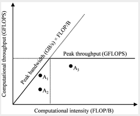 |
|---|
| Roofline model for analyzing GPU efficiency |
The axes meanings:
x-axisis the computational intensity measured inFLOP/B. This quantity is determined by how the application is written.y-axisis the computational throughput, i.e. obtained by multiplying the computational intensity by the maximum memory bandwith of our hardware device (a fixed constant)- The peak throughput horizontal line is the hard cap of the hardware on the peak throughput it can support
The sloping line labelled peak bandwidth represents the hardward limit of the memory bandwidth. The slope is obtained by multipling the current position on the x-axis by the maximum memory bandwidth (say 1555GB/s in the example above), which gives us a slope. We cannot have any point above this line because it would require a memory bandwidth that exceeds the hardware limits.
A point on the plot represents an application with its computational intensity (FLOPS / byte accessed) and computational throughput (FLOPS / s). Note that in real applications, these are measured using programs like NVIDIA NSight using hardware counters. The position of the point relative to the lines tells us its efficiency:
- Points can only be below the two lines, as we cannot exceed hardware limits
- Points closer to the lines are more efficient, as we are nearing hardware limits
Based on the diagram:
- Point is compute bound - it is already quite computationally intensive and near the peak computational throughput, so we need a more powerful GPU to improve it further.
- Point is inefficient - neither memory nor compute bound. It can be improved by improving the memory bandwidth utilization.
- Point is memory bound - it is utilizing memory bandwidth effectively but the compute intensity can be improved. e.g. To fully utilize the
19,500 GLOPSfrom the A100, we need to increase compute efficiency to19,500 (GFLOP/s) / 1,555 (GB/s) = 12.5 FLOP/B. This means that for each single precision floating point number accessed, we need to perform50 FLOPS! This can be achieved for certain applications like matrix multiplication.
CUDA Memory Types
There are different memory types on a GPU with different uses:
- Registers
- Registers are on-chip memory, which means very short latency, high bandwidth access
- Highly limited number of registers per SMs, using too many in kernel code can result in low occupancy
- Allocated to individual threads - each thread can only access its own registers
- Shared memory
- Also on-chip memory, but it resides outside of the Processing Unit
- Accessing data requires a memory load (as opposed to registers), so it is slower than registers, but the memory load is much faster than global memory as it is on-chip
- Allocated to thread blocks - all threads in a block can access shared memory variables
- Global memory
- All threads can access
- Off-chip memory, so relatively high latency and low bandwidth access
- Local memory
- Placed in global memory and has similar access latency
- Not shared across threads
- Each thread has its own section of global memory that it uses as its own private local memory that is private to the thread but cannot be allocated in registers
- e.g. statically allocated arrays
Efficient GPU code requires us to make full use of registers whenever possible:
- Access bandwidth of registers is at least 2 orders of magnitude higher than global memory
- When a variable is stored in registers, its access no longer consume off-chip global memory bandwith, which is reflected as an increased compute to global memory access ratio
- Each access to registers involves fewer instructions than access to global memory due to built-in register operands.
- e.g.
fadd r1, r2, r3directly adds values in registersr2, r3and stores it intor1. There is no loading step - But if the first operand is in the global memory, we need to do an extra loading step
load r2, r4, offset fadd r1, r2, r3 - e.g.
- The energy consumed for accessing a value in the register file is an order of magnitude lower than accessing the value from global memory.
CUDA Syntax
We can declare variables and reside them in the intended type of memory based on our application design.
Scope. Scope identifies the set of threads than can access a variable. If the scope is a single thread, a private version of the variable is created for each thread.
Lifetime. The lifetime is the portion of a program's execution duration when the variable is available, If the lifetime is within a grid's execution, it must be declared within the kernel function. When the kernel is executed multiple times, the value is not maintained across these invocations. If the lifetime is entire application, it must be declared outside of any function body.
Automatic Scalar Variables. All automatic scalar variables declared in the kernel and device functions are automatically placed into registers. This means that a private copy of that variable in generated for every thread that executes the kernel function.
- Scope: Thread
- Lifetime: Grid
Automatic array variables. These are array variables defined in kernel code, such as float buf[128]. Note that the array size must be specified at compile time. These are put into local memory (part of global memory), so access is very slow. In practice, these are seldom used.
- Scope: Thread
- Lifetime: Grid
Shared Memory variables. These are declared in the kernel function and put into shared memory. The scope of a shared variable is in a thread block, so all threads in a block see the same version of a shared variable (and can read and write to it). A private version of the variable is created for each block during kernel execution. Accessing shared variables from the shared memory is extremely fast and highly parallel, and it is a good way for threads in a block to communicate with each other.
- Declaration:
__device__ __shared__ int SharedVar; - Scope: Block
- Lifetime: Grid
Constant Memory variables. These are declared in the host code outside of any function body, and its values cannot be changed by kernel function code. The name is indicative: its usually used for global constants like model parameters or for things like a fixed convolution filter. Constant variables are stored in global memory but are cached for extremely fast and parallel access. The total size of constant variables in an application is limited to 65,536 bytes.
- Declaration:
__device__ __constant__ int ConstVar; - Scope: Grid
- Lifetime: Application
Global Memory variables. These are placed in global memory where access is slow. The advantage of global memory is that it is accessible by all threads and the contents persist throughout the entire application. So it is a way for threads to collaborate across blocks. However, because there is no barrier synchronization method for threads across blocks, usually global variables are used to pass information from one kernel invocation to another kernel.
- Declaration:
__device__ int GlobalVar; - Scope: Grid
- Lifetime: Application
Tiling
The intrinsic memory tradeoff in CUDA is that global memory is large but slow, and shared memory is small but fast. Hence a good strategy is to partition the data into subsets called tiles so that each tile fits into the shared memory.
Consider the matrix multiplication example in chapter 3 where each thread computes one value of the output matrix P = M dot N, and thus access one row of M and one column of N.
- For brevity, define as
M[y*Width + x], asN[y*Width + x], asP[y*Width + x] - Suppose
Width=4and our block size is2 x 2
Now observe that there are duplicate global memory accesses across threads in a block:
- is accessed for computing both and
- is accessed for computing both and
- And so on
Instead of accessing global memory twice, we could have accessed it once, loaded it into shared memory, and then have threads read from shared memory thereafter (almost negligible cost compared to accessing global memory). In fact, a given value (like ) will be accessed block_size times for a given block, so the larger our block size, the more efficient our memory access can be.
We are limited by the size of shared memory, so we need to further tile M and N matrices so that it will fit into shared memory. For simplicity, consider tiling M and N into 2 x 2 tiles also.
Our strategy will now be like so:
- Initialize
2 x 2shared variablesMdsandNds - Load a tile of
MintoMds:- For e.g. the first tile would be
- Load a tile of
NintoNds:- For e.g. the first tile would be
- Launch threads to accumulate partial dot product into thread-specific
Pvalue:- Instead of reading from
MandN, we read the required variables fromMdsandNdsinstead - e.g. computes
- Note that this is a partial dot product for , we need to accumulate to it again
- Instead of reading from
- Move on to the next tile and accumulate to
Pvalueagain:- e.g. Second tile is
- e.g. Second tile is
Note that with this tiling strategy, we will need to do this in multiple steps (or phases) for a given block. In general, we need Width / TILE_WIDTH phases to complete the matrix multiplication.
A tiled matmul kernel
Now we can tackle the matmul kernel.
# define TILE_WIDTH 16
__global__ void matrixMulKernel(float* M, float* N, float* P, int Width) {
__shared__ float Mds[TILE_WIDTH][TILE_WIDTH];
__shared__ float Nds[TILE_WIDTH][TILE_WIDTH];
int bx = blockIdx.x; int by = blockIdx.y;
int tx = threadIdx.x; int ty = threadIdx.y;
// Identify P[Row, Col] to work on
int Row = by * TILE_WIDTH + ty;
int Col = bx * TILE_WIDTH + tx;
float Pvalue = 0;
for (int ph = 0; ph < Width/TILE_WIDTH; ++ph) {
// Load M, N into shared memory
Mds[ty][tx] = M[Row*Width + ph*TILE_WIDTH + tx];
Nds[ty][tx] = N[(ph*TILE_WIDTH + ty)*Width + Col];
__syncthreads();
for (int k = 0; k < TILE_WIDTH; ++k) {
Pvalue += Mds[ty][k] * Nds[k][tx];
}
__syncthreads();
}
P[Row*Width + Col] = Pvalue;
}
Notes on the above:
Mds, Ndsare shared variables that are common for all threads in a block- Since each thread is working on one element of output
P, we findRowandColrespectively (to computeP[Row, Col])- Note that the algorithm assumes each block computes exactly one tile, so
TILE_WIDTH = BLOCK_SIZE - Therefore
Row = by * TILE_WIDTH + ty - And
Col = bx * TILE_WIDTH + tx
- Note that the algorithm assumes each block computes exactly one tile, so
Now we tackle the for loop part which loops through the phase counter ph.
- Recall that each phase uses one tile of
Mand one tile ofN. - The phase counter
phtells us how many phases we have already processed
Loading Data into Shared Memory
For each phase, we first load data into shared memory:
- Each thread loads one value of
Mnad one value ofNinto shared memory - Since we have
TILE_WIDTH x TILE_WIDTHnumber of threads per block, in each phase we load this many elements intoMdsandNdsrespectively
Which data should each thread load?
- For
M:- Note that
Rowalready gives us the row ofMto be loaded for this thread (constant across phases) - The beginning column for this block and phase is
ph * TILE_WIDTH, because we have processedphnumber of tiles to the left - So we want
M[Row, ph*TILE_WIDTH], which is indexed asM[Row*Width + ph*TILE_WIDTH + tx]in row major form
- Note that
- For
N:Colalready gives us the column ofNto be loaded for this thread (constant across phases)- The beginning row for this block and phase is
ph * TILE_WIDTH - So we want
N[ph*TILE_WIDTH + ty, Col], which is indexed asN[(ph*TILE_WIDTH + ty)*Width + Col]
Finally, we call __syncthreads() barrier synchronization. This is necessary because for the computation phase, each thread requires values of Mds,Nds that other threads have loaded for it. Hence we must make sure all threads have loaded into shared memory before we proceed to compute.
- This is called read-after-write synchronization - we require data to be written before we can read from it
- Also called true dependence because there is truly a dependence from the reader on the written data
Computation Phase
Now we have loaded the requisite data into Mds and Nds, we can accumulate into Pvalue. The tiled matmul is such that we accumulate into Pvalue as though we were just doing a simple dot product between Mds and Nds. This compute phase is very fast as we are reading from shared memory.
Finally, another __syncthreads() is called. This is to ensure that computation has completed before we start loading values into Mds and Nds in the next phase, overwriting their values.
- This is called write-after-read synchronization - threads must wait for data to be read by all threads that need it before overwriting it
- Another name is false dependence. The dependence is false because the writing thread actually does not need any data from the reading thread - the dependence occurs purely because they are sharing the same memory location.
Summary
The savings from tiled matmul is significant. With 16 x 16 tiles, we reduce global memory access by a factor of 16, which brings our 0.25 FLOP/B to 4 FLOP/B. There are further optimizations we can make later.
Boundary Checks
In the previous section, we assume that Width is a multiple of TILE_WIDTH. This section extends it to handle arbitrary matrix sizes. As with before, we need to add boundary checks to avoid accessing non-existent values or even accessing wrong values that corrupt the final output.
The modified kernel code is shown (only the for loop part):
float Pvalue = 0;
for (int ph = 0; ph < ceil(Width/(float) TILE_WIDTH); ++ph) {
if ((Row < Width) && (ph*TILE_WIDTH+tx) < Width)
Mds[ty][tx] = M[Row*Width + ph*TILE_WIDTH + tx];
else Mds[ty][tx] = 0.0f;
if ((ph*TILE_WIDTH+ty) < Width && Col < Width)
Nds[ty][tx] = N[(ph*TILE_WIDTH+ty)*Width + Col];
else Nds[ty][tx] = 0.0f;
__syncthreads();
for (int k = 0; k < TILE_WIDTH; ++k) {
Pvalue += Mds[ty][k] * Nds[k][tx];
}
__syncthreads();
}
if (Row < Width) && (Col < Width)
P[Row*Width + Col] = Pvalue;
For boundary checks on M:
- As we recall, the
yandxelement accessed areRowandph*TILE_WIDTH + txrespectively - Hence we just need to check if both of these are less than
Width
For boundary checks on N:
- The
yandxelement accessed are(ph*TILE_WIDTH+ty)andColrespectively - Hence we just need to check if both of these are less than
Width
For accessing M and N, if we are accessing an out of bounds value, simply load 0.0 into Mds and Nds respectively. This will ensure that when accumulating into Pvalue, using an out of bound value will result in adding 0.0 and hence not affect the final output.
Finally when assigning values into P, we just check if Row, Col are within bounds.
Impact of Memory Use on Occupancy
Earlier on we saw that register usage can reduce occupancy. Similarly, using too much shared memory can reduce the number of blocks assigned and hence reduce occupancy.
For example, an A100 can have up to 164KB of shared memory per SM and support a maximum of 2048 threads per SM.
- This means that to use up all thread slots, a thread block cannot use more than an average of
164 KB / 2048 threads = 82B / thread
For our tiled matmul example:
- Each block has
TILE_WIDTH * TILE_WIDTHthreads per block - Each block uses
4B * TILE_WIDTH * TILE_WIDTHshared memory forMdsandNdsrespectively - So it uses
8Bper thread, which is less than82Band we are fine
But consider a kernel that uses 32KB of shared memory, and each block has 256 threads.
- Then each thread uses on average
32KB / 256 = 128B. This exceeds the82B/threadlimit. - So we can only launch at most
164KB / 128B = 1.3k threads, which is around60%occupancy
Dynamic sizing of shared memory
Since the size of shared memory on an SM is device specific, we want the host code to dynamically adjust the TILE_WIDTH and hence amount of shared memory used by a kernel.
- This can be done using
cudaGetDeviceProperties, and usingdevProp.sharedMemPerBlockto give the amount of shared memory available in each SM.
Unfortunately, we cannot specify Mds and Nds as before using TILE_WIDTH, because the value of TILE_WIDTH must be available at compile time. If we want to change this value, we must recompile the code.
The workaround for such a scenario is to use extern __shared__ Mds_Nds[]; inside the kernel code. This allows for a dynamically allocated shared array.
- However, since we only have one merged array, we'll need to manually define where
Mdsends andNdsstarts - We also need to linearize our access to the array
At runtime, we can dynamically configure the amount of shared memory for each block using the third configuration parameter for a kernel call:
size_t size = calculate_appropriate_SM_usage(devProp.sharedMemPerBlock, ...);
matrixMulKernel<<<dimGrid,dimBlock,size>>>(Md, Nd, Pd, Width, size/2, size/2);
Notes:
- Note that
size_tis a built-in type for declaring a variable to hold the size information for dynamically allocated data structures, in number of bytes. - Also note that we pass
size/2for the size ofMdsandNdsrespectively
The kernel code can then be modified to accommodate the new structure:
#define TILE_WIDTH 16
__global__ void matrixMulKernel(float* M, float* N, float* P, int Width,
unsigned Mdz_sz, unsigned Nds_sz) {
extern __shared__ char float Mds_Nds[];
float *Mds = (float*) Mds_Nds;
float *Nds = Mds_Nds + Nds_sz;
}
Note that we would need to use linearized accesses to Mds and Nds. e.g. Mds[ty][tx] becomes Mds[ty*TILE_WIDTH+tx].
Exercises
- Consider matrix addition. Can one use shared memory to reduce the global memory bandwidth consumption? Hint: Analyze the elements that are accessed by each thread and see whether there is any commonality between threads.
No - each element of input matrices A + B are accessed exactly once, so no memory savings.
- Draw the equivalent of Fig. 5.7 for a 8×8 matrix multiplication with 2×2 tiling and 4×4 tiling. Verify that the reduction in global memory bandwidth is indeed proportional to the dimension size of the tiles.
- With 2x2 tiling, there are 4 phases, so each element gets accessed from global memory 4x
- With 4x4 tiling, there are 2 phases, so each element gets accessed from global memory 2x
- So the reduction in memory bandwidth is proportional to the tile size
With 2x2 tiling, each element gets accessed twice per phase. With 4x4 tiling, each element gets accessed 4x per phase. So the reduction in global memory bandwidth is scaled accordingly.
- What type of incorrect execution behavior can happen if one forgot to use one or both __syncthreads() in the kernel of Fig. 5.9?
This is the tiled matrix multiplication code.
- If we miss the first
__syncthreads, we could get "read-before-write" situations where another thread tries to load the values ofMdsorNdsbefore it is written. This leads to wrong outputs. - If we miss the second
__syncthreads, we could get "write-before-read" situations, where another thread has already overwritten the values ofMdsorNdsin the next phase before we have read from it. This leads to wrong outputs.
- Assuming that capacity is not an issue for registers or shared memory, give one important reason why it would be valuable to use shared memory instead of registers to hold values fetched from global memory? Explain your answer.
Threads in the same block can access the shared memory, so we can benefit as long as our application requires multiple threads to access the same values. Registers are private to each thread and we cannot benefit.
- For our tiled matrix-matrix multiplication kernel, if we use a 32×32 tile, what is the reduction of memory bandwidth usage for input matrices M and N?
32x
- Assume that a CUDA kernel is launched with 1000 thread blocks, each of which has 512 threads. If a variable is declared as a local variable in the kernel, how many versions of the variable will be created through the lifetime of the execution of the kernel?
512,000
- In the previous question, if a variable is declared as a shared memory variable, how many versions of the variable will be created through the lifetime of the execution of the kernel?
1000
- Consider performing a matrix multiplication of two input matrices with dimensions N×N. How many times is each element in the input matrices requested from global memory when: a. There is no tiling? b. Tiles of size T×T are used?
Easier to reason about total number of accesses:
- With no tiling, each thread accesses
2Nelements and there areNxNthreads, so2N^3 - With tiling, each block accesses
2TNelements, and there areN/T * N/Tblocks, so2N^3/Taccesses
- A kernel performs 36 floating-point operations and seven 32-bit global memory accesses per thread. For each of the following device properties, indicate whether this kernel is compute-bound or memory-bound. a. Peak FLOPS=200 GFLOPS, peak memory bandwidth=100 GB/second b. Peak FLOPS=300 GFLOPS, peak memory bandwidth=250 GB/second
The computational intensity is 36 FLOP / (7 * 4B) = 1.3 FLOP/B
- With peak memory bandwidth of
100 GB/s, our throughput is1.3 (FLOP/B) * (100 GB/s) = 130 GFLOPS. This means we are memory bound as we are not hitting peak FLOPS - With peak memory bandwidth of
250 GB/s, our throughput is1.3 (FLOP/B) * (250 GB/s) = 325 GLOPS. This means we are compute bound as we have hit peak FLOPS
- To manipulate tiles, a new CUDA programmer has written a device kernel that will transpose each tile in a matrix. The tiles are of size BLOCK_WIDTH by BLOCK_WIDTH, and each of the dimensions of matrix A is known to be a multiple of BLOCK_WIDTH. The kernel invocation and code are shown below. BLOCK_WIDTH is known at compile time and could be set anywhere from 1 to 20.
01 dim3 blockDim(BLOCK_WIDTH, BLOCK_WIDTH);
02 dim3 gridDim(A_width/blockDim.x, A_height/blockDim.y);
03 BlockTranspose<<<gridDim, blockDim>>>(A, A_width, A_height);
04 __global__ void
05 BlockTranspose(float* A_elements, int A_width, int A_height)
06 {
07 __shared__ float blockA[BLOCK_WIDTH][BLOCK_WIDTH];
08 int baseIdx = blockIdx.x * BLOCK_WIDTH + threadIdx.x;
09 baseIdx += (blockIdx.y * BLOCK_WIDTH + threadIdx.y) * A_width;
10 blockA[threadIdx.y][threadIdx.x] = A_elements[baseIdx];
11 A_elements[baseIdx] = blockA[threadIdx.x][threadIdx.y];
12 }
a. Out of the possible range of values for BLOCK_WIDTH, for what values of BLOCK_WIDTH will this kernel function execute correctly on the device?
The code works like so:
- Each thread handles an element of
A - The tile / block size is
BLOCK_WIDTH - For each thread:
threadIdx.xandthreadIdx.ygive thex,ycoordinates within a block- We wish to swap these elements by temporarily assigning into
blockA
- What is the index of the element we are accessing?
- The
yindex inAwould beblockIdx.y * BLOCK_WIDTH + threadIdx.y - The
xindex inAwould beblockIdx.x * BLOCK_WIDTH + threadIdx.x - So the serialized form is
y*A_width + xas shown in the code
- The
The problem with the code is that we have a potential "write-before-read" situation in line 10-11:
- Consider
thread1: threadIdx.y=i, threadIdx.x=jandthread2: threadIdx.y=j, threadIdx.x=iwhich are two threads in mirror coordinates to each other - It is possible that
thread1completes the transpose operation beforethread2and writes intoA_elementsbeforethread2reads - Then, we end up with
thread1andthread2writing the same value into their designated slots which is incorrect
The only BLOCK_WIDTH value which works is 1.
b. If the code does not execute correctly for all BLOCK_SIZE values, what is the root cause of this incorrect execution behavior? Suggest a fix to the code to make it work for all BLOCK_SIZE values.
Add a __syncthreads() between lines 10 and 11.
- Consider the following CUDA kernel and the corresponding host function that calls it:
01 __global__ void foo_kernel(float* a, float* b) {
02 unsigned int i = blockIdx.x * blockDim.x + threadIdx.x;
03 float x[4];
04 __shared__ float y_s;
05 __shared__ float b_s[128];
06 for (unsigned int j = 0; j < 4; ++j) {
07 x[j] = a[j * blockDim.x * gridDim.x + i];
08 }
09 if (threadIdx.x == 0) {
10 y_s = 7.4f;
11 }
12 b_s[threadIdx.x] = b[i];
13 __syncthreads();
14 b[i] = 2.5f * x[0] + 3.7f * x[1] + 6.3f * x[2] + 8.5f * x[3]
15 + y_s * b_s[threadIdx.x] + b_s[(threadIdx.x + 3) % 128];
16 }
17
18 void foo(int* a_d, int* b_d) {
19 unsigned int N = 1024;
20 foo_kernel<<< (N + 128 - 1) / 128, 128 >>>(a_d, b_d);
21 }
a. How many versions of the variable i are there?
i is private to each thread, so 1024 copies.
b. How many versions of the array x[] are there?
x[4] is a local memory variable and private to each thread, so 1024 copies.
c. How many versions of the variable y_s are there?
y_s is a shared memory variable, one per block, so 8 copies.
d. How many versions of the array b_s[] are there?
b_s is also shared memory, so 8 copies.
e. What is the amount of shared memory used per block (in bytes)?
We have (128 + 1) * 4B = 516B.
f. What is the floating-point to global memory access ratio of the kernel (in OP/B)?
There are 6 memory accesses, so 24B in each thread:
- Line 7 has
4loads - Line 12 has
1load - Line 14 has
1store
There are 10 floating point operations on lines 14 and 15:
5multiplications5additions
So FLOP/B is 10 / 24 = 0.42 FLOP/B.
- Consider a GPU with the following hardware limits: 2048 threads/SM, 32 blocks/SM, 64K (65,536) registers/SM, and 96 KB of shared memory/SM. For each of the following kernel characteristics, specify whether the kernel can achieve full occupancy. If not, specify the limiting factor.
a. The kernel uses 64 threads/block, 27 registers/thread, and 4 KB of shared memory/block.
Checks:
- Total threads:
64 threads/block * 32 blocks = 2048. Hits thread limits ✔ - Shared memory: given shared memory limits, we can only have
96KB / 4KB = 24 blocks. So occupancy can only be 75%. ✖ - Registers:
27 * 2048 = 55,296. Within limits ✔
Cannot reach full occupancy due to shared memory usage.
b. The kernel uses 256 threads/block, 31 registers/thread, and 8 KB of shared memory/block.
Checks:
- Total threads:
256 threads/block * 8 blocks = 2048. Hits thread limits ✔ - Shared memory: given shared memory limits, we have
96KB / 8KB = 12 blocks. So we can have 8 blocks no problem. ✔ - Registers:
31 * 2048 = 63,488. Within limits ✔
Can reach full occupancy.
Performance Considerations
This chapter goes deeper into off chip memory (DRAM) and discusses memory coalescing and memory latency hiding. It also discusses thread granularity coarsening.
Memory Coalescing
One of the most important factors in CUDA kernel performance is accessing data in the global memory. This chapter further discusses memory coalescing techniques to move data between global memory and shared memory or registers efficiently.
Global memory is implemented with DRAM:
- Access latency to a bit in DRAM is relatively slow (tens of nanoseconds)
- Because of this slowness, DRAM is designed to use parallelism to increase the memory access throughput
Each time a DRAM location is accessed, a range of consecutive locations nearby are accessed. Once detected by the sensors, the data from all these locations can be transferred to the processor.
- These consecutive locations assessed is known as DRAM bursts
- Making use of these consecutive and simultaneous accesses can allow us to improve memory access throughput
When a warp of threads is launched, all threads in the warp execute the same instruction at the same point in time. The hardware detects whether the threads are accessing consecutive memory locations.
- Thus, the best access pattern is for threads in a warp to access consecutive data locations in global memory
- We say that the hardware coalesces the accesses into a consoliated access to consecutive DRAM locations
Recall that multidimensional data are linearized according to the row-major convention and stored into memory space. The read accesses are coalesced if consecutive threads in a warp are assigned to consecutive memory elements in this row major storage format.
Row Major
Consider the following matrix multiplication code in which each thread computes one element of the output matrix P without tiling:
unsigned int row = blockIdx.y*blockDim.y + threadIdx.y;
unsigned int col = blockIdx.x*blockDim.x + threadIdx.x;
if (row < Width && col < Width) {
float Pvalue = 0.0f;
for (unsigned int k = 0; k < Width; ++k) {
Pvalue += N[row*Width + k]*M[k*Width + col];
}
P[row*Width + col] = Pvalue;
}
Notice that memory accesses to M are coalesced because:
- The index of
Misk * Width + col kandWidthhave the same values across all threads in a warpcol = blockIdx.x * blockDim.x + threadIdx.x, which means that consecutive threads (with incrementingthreadIdx.x) will access consecutive elements
Column Major
Now suppose the matrix is stored in column major format instead. Now the code adjusts to the following:
unsigned int row = blockIdx.y*blockDim.y + threadIdx.y;
unsigned int col = blockIdx.x*blockDim.x + threadIdx.x;
if (row < Width && col < Width) {
float Pvalue = 0.0f;
for (unsigned int k = 0; k < Width; ++k) {
Pvalue += N[row*Width + k]*M[col*Width + k];
}
P[row*Width + col] = Pvalue;
}
Observe that the index to M changed from k*Width + col to col*Width + k. This is because in the column major format, elements that were previously in adjacent columns to each other are now in adjacent rows. Hence the indexing to M is swapped to reflect this.
Now we can see that we have lost the coalesced access to M:
- The indexing to
Mis nowcol*Width + k - Consecutive threads still have consecutive values of
col - But
colis now multiplied byWidth, meaning that consecutive threads access values that areWidthapart, which can be very far
Corner Turning
This is a method to create coalesced memory accesses even when the computation is not naturally amenable to it. The idea is to read from global memory into shared memory in a coalesced manner, then do the unfavourable access pattern from the cheap shared memory instead.
Suppose we are in the tiled matrix multiplication example. First, we do a coalesced read from M into Mds for our tile by swapping the row and column. The elements can be arranged in Mds in either row or column major format, it does not matter. Then, we can do fast reads from Mds to do the matrix multiplication for our tile.
Hiding Memory Latency
DRAM bursting is a form of parallel organization: multiple locations are accessed in the DRAM core array in parallel. There are two more ways of parallel organization: banks and channels. A single processor may have 8 channels. Each channel has a bus that accesses many banks.
The bus transfers data from the banks back to the processor. The data transfer bandwidth of the bus is defined by its width and clock frequency. Modern DDR buses perform two data transfers per clock cycle.
- e.g. A 64-bit DDR bus with clock frequency of 1 GHz has a bandwidth of
8B * 2 * 1 = 16GB/s.
For each channel, we need many banks in order to fully utilize the data transfer bandwidth of the bus. Why?
- Recall earlier that the data access latency is slow, because it takes time for cells to share their stored charge with the sensing amplifier
- Once the sensing amplifier has completed its work, the burst data is delivered through the bus (this part is relatively much faster)
- If we only have a single bank, there is a long latency waiting for the sensing amplifier while the bus sits idle
- If we have multiple buses, we can trigger multiple read accesses to different banks in close succession in an async manner
- When each bank has been sensed, the delivery of burst data can be tightly packed and fill up the idle time
In general, if the ratio of cell array access latency / data transfer time = R, then we need to have at least R + 1 banks to fully utilize the data transfer bandwidth of the bus.
- Note that we need more than
Rbecause of bank conflict. Since each bank can only serve one data access at a time (each bank can store multiple data points), if multiple threads need to access the same bank for data, there is a conflict. So having more banks help to reduce the probability of bank conflict
There is an important connection between occupancy and parallel access to DRAM data. As we saw earlier, maximizing occupancy ensures that we have enough threads on the SMs to hide long memory access latencies. In this section, we see another distinct advantage of maximizing occupancy - having many threads access different memory locations allows us to fully utilize the memory transfer bandwidth of the buses. That is, if the memory accesses are well distributed across channels and banks.
Practically, the distribution of data across channels and banks is in an interleaved data distribution. Suppose we have a toy example:
4channels2banks per channel- Each bank stores
2consecutive floats
Now suppose we are doing a tiled matrix multiplication between two 4 x 4 matrices M @ N, where we set the tile width to 2.
The storage of M is like so (referring to the linearized index):
- Channel 0
- Bank 0:
M[0], M[1] - Bank 1:
M[8], M[9]
- Bank 0:
- Channel 1
- Bank 0:
M[2], M[3] - Bank 1:
M[10], M[11]
- Bank 0:
- Channel 2
- Bank 0:
M[4], M[5] - Bank 1:
M[12], M[13]
- Bank 0:
- Channel 3
- Bank 0:
M[6], M[7] - Bank 1:
M[14], M[15]
- Bank 0:
As we can see, consecutive elements of our data arrays is first put into bank 0 of all the channels. It then moves on to bank 1 of all the channels. If there is more data, we will wrap back around to bank 0 again. The breadth-first distribution across channels helps ensure that even when the amount of data is small, we have good distribution of data across channels and banks.
Now for the matrix multiplication, we can verify that in phase 0 of the tiled matrix multiplication, these are the elements of M requested by each block:
Block 0,0:M[0], M[1], M[4], M[5]Block 0,1:M[0], M[1], M[4], M[5]Block 1,0:M[8], M[9], M[12], M[13]Block 1,1:M[8], M[9], M[12], M[13]
This is a bit tedious so will not elaborate on how these were derived. But basically, we can see that we access both banks of channels 0 and 2 for phase 1. So we are utilizing 50% of the channels. With multiplication of larger matrices, we can fully utilize all channels and buses.
Thread Coarsening
So far, we have focused on kernels where work is parallelized across all threads at the finest granularity. For e.g. in the matrix multiplication example, each thread is assigned one element in the output matrix P. The advantage of parallelizing at the finest granularity is that it enhances transparent scalability - if the hardware has enough resources to run all the work in parallel, then we have maximized the parallelism.
However, if the hardware does not have enough resources to run all the work at once, then a queue is formed up, and the parallel work becomes sequential. In this case, there is a price to be paid for such aggressive parallelism, such as:
- redundant loading of the same data by different blocks
- redundant work
- syncrhonization overhead
When the threads are executed in parallel, this price is often well worth it. But if the hardware ends up serializing the work as a result of insufficient resources, this price may have been paid unnecessarily. It may thus be worthwhile to reduce the amount of parallelism by having each thread do more work, in exchange for reducing the price that we pay.
One such technique is called thread coarsening. We can see a good example in the tiled matrix multiplication example. For calculating a given tile in the output matrix P, each thread block must load its own copy of the input tiles of matrix M. However, this means that the same tile of input matrix M will be loaded redundantly by different thread blocks and incurring access to global memory.
More concretely, consider that we are computing rows of P from P[i, :] to P[j, :].
- One thread block may be computing
P[i, k1] to P[j, k2] - One thread block may be computing
P[i, k2] to P[j, k3] - But notice that to do this computation, they all have to access
M[i, k1] to M[j, k2]in one of their phases - It may make more sense for a single thread block to compute a few adjacent
Ptiles at once, and thus load this slice of matrixMonly once and reduce redundant memory accesses
Here we can dive into the thread coarsening matrix multiplication kernel:
#define TILE_WIDTH 32
#define COARSE_FACTOR 4
__global__ void matrixMulKernel(float* M, float* N, float* P, int width) {
__shared__ float Mds[TILE_WIDTH][TILE_WIDTH];
__shared__ float Nds[TILE_WIDTH][TILE_WIDTH];
int bx = blockIdx.x; int by = blockIdx.y;
int tx = threadIdx.x; int ty = threadIdx.y;
int row = by * TILE_WIDTH + ty;
int colStart = bx * TILE_WIDTH * COARSE_FACTOR + tx;
float Pvalue[COARSE_FACTOR];
for (int c = 0; c < COARSE_FACTOR; ++c) {
Pvalue[c] = 0.0f;
}
for (int ph = 0; ph < width/TILE_WIDTH; ++ph) {
Mds[ty][tx] = M[row*width + ph*TILE_WIDTH + tx];
for (int c = 0; c < COARSE_FACTOR; ++c) {
int col = colStart + c * TILE_WIDTH;
Nds[ty][tx] = N[(ph * TILE_WIDTH + ty) * width + col];
__syncthreads();
for (int k = 0; k < TILE_WIDTH; ++k) {
Pvalue[c] += Mds[ty][k] * Nds[k][tx];
}
__syncthreads();
}
}
for (int c = 0; c < COARSE_FACTOR; ++c) {
int col = colStart + c * TILE_WIDTH;
P[row * width + col] = Pvalue[c];
}
}
Let's unpack the code above. Notice that instead of each thread block processing one tile of the output P matrix, now one thread block will process COARSE_FACTOR = 4 adjacent tiles of P
- Therefore, each thread now processes
4cells instead of1cell
First we identify row and colStart:
rowis the row ofPthat we are computing. This is as per normalcolStartis the start of the column that we are computing. Because each thread is now doing4cells, we multiply byCOARSE_FACTORto start further down. It is also the "start" because there are 4 cells to compute, and this variable indicates the first cell.
Initialize Pvalue: instead of one float, we have an array of 4 floats.
Now the main loop:
- The outer loop is over phases, which is as per previous. Each phase loads a new tile of
M(by moving rightwards) and a new tile ofN(by moving downwards) to compute the samePtile in a tiled manner. - Notice that we load a tile of
Mfor this block that will be reused across multiple loops of the coarsening loop overc.- The way
Mis loaded is as per normal - we locate the correctrow, and the column is determined byph * TILE_WIDTH + tx
- The way
- The coarsening loop is where things are interesting:
- For a given value of
c, we are working on one tile ofN - Each iteration of the loop moves us in a stride of
TILE_WIDTHto the right, as reflected by the waycolis computed ascolStart + c * TILE_WIDTH - e.g. a given thread may compute
col = 0, 32, 64, 96instead ofcol = 0, 1, 2, 3 - Once we have computed
colto account for coarsening, the indexing intoNis as per previous
- For a given value of
So we see that for the same M tile that is loaded, we reuse it COARSE_FACTOR times for different N tiles. Thread coarsening is a common technique that can led to substantial performance improvements.
Pitfalls
There are some potential pitfalls for thread coarsening:
- Not to apply optimization when it is unnecessary. Thread coarsening is only beneficial when there is a price paid for parallelization, such as redundant data loading. It will not help when there is no price paid.
- Apply too much coarsening such that hardware resources become underutilized. By applying coarsening, we reduce the amount of parallelism exposed and can lead to underutilisation.
- Third pitfall is that our coarsened kernel ends up using more resources which can hurt occupancy, for example, by using more registers per thread or more shared memory per thread block.
Checklist of optimizations
- Maximizing occupancy
- Idea: more parallel memory accesses to hide DRAM latency
- Strategy: tune parameters like threads per block, shared memory per block, registers per thread to maximize occupancy
- Enabling coalesced global memory accesses
- Idea: less global memory traffic and better utilization of DRAM burst to efficiently read data
- Strategies:
- Transfer from global to shared memory in a coalesced manner and perform uncoalesced accesses in shared memory
- Rearrange mapping of threads to data
- Rearrange layout of data
- Minimize control divergence
- Idea: Higher SIMD efficiency and have less idle cores during SIMD execution
- Strategies:
- Rearrange mapping of threads to work and / or data
- Rearrange layout of data
- Tiling of reused data
- Idea: Less global memory traffic by reusing tiles
- Strategies:
- Place reused data in shared memory or registers so that we only read from global memory once
- Privatisation
- Idea: Less contention of writes to a shared copy of data and serialization of atomic updates
- Strategy:
- Apply partial updates to a private copy of the data and then updataing the universal copy when done
- Thread coarsening
- Idea: Less redundant work, divergene and global memory traffic
- Strategy:
- Assign multiple units of parallelism to each thread to reduce the price of parallelism when unnecessarily incurred
Exercises
- Write a matrix multiplication kernel function that corresponds to the design illustrated in Fig. 6.4.
Fig 6.4 is the corner turning example. Suppose we have matrices M x N = P. For simplicity, we assume square matrices of Width.
The access to M remains the same as normal tiled matrix multiplication, but we want to change the way N is loaded into shared memory, since the assumption is that N is stored in column major format.
Doing a recap: each block computes a tile of P. Let T denotes the TILE_WIDTH. The rows and columns are determined by the current values of by and bx respectively:
- The first row of the block is
by * T - The first column of the block is
bx * T tyandtxgives us the coordinate of the exact element within the block
Now let's focus on N. Here we need to distinguish between the logical indexing into N (call it N_logical) and the indexing into N based on how it is stored (column major, call it N_stored). We start with the logical view:
- Each phase of the tiled matmul moves us downward on
N - So we start at row
ph * Tand work downwards - The columns are fixed as
bx * Ttobx * (T+1) - 1
Since N is stored in column major, we need to swap the indexing when referring to N_stored. So:
- We start at row
bx * T(denotedN_rowstartin code) - We start at column
ph * T(denotedN_colstartin code)
Now we have found the correct coordinates of the tile within N. This is where it gets tricky: we want to read the elements of this tile in a coalesced way, such that incrementing tx by 1 reads the next element in the linearized array.
- So the first element is
N_rowstart * Widthcorresponding toN_logical[ph*T, bx*T] - Second element is
N_rowstart * Width + 1corresponding toN_logical[ph*T + 1, bx*T]etc. - This means that we will be reading in the transpose of this N tile, and we need to transpose it again when loading into
Ndsso that we get the correct tile when doing the final multiplication
Hopefully this analysis sheds some light on the code below.
# define TILE_WIDTH 16
__global__ void matrixMulKernel(float* M, float* N, float* P, int Width) {
__shared__ float Mds[TILE_WIDTH][TILE_WIDTH];
__shared__ float Nds[TILE_WIDTH][TILE_WIDTH];
int bx = blockIdx.x; int by = blockIdx.y;
int tx = threadIdx.x; int ty = threadIdx.y;
// Identify P[Row, Col] to work on
int Row = by * TILE_WIDTH + ty;
int Col = bx * TILE_WIDTH + tx;
float Pvalue = 0;
for (int ph = 0; ph < Width/TILE_WIDTH; ++ph) {
// Load M, N into shared memory
Mds[ty][tx] = M[Row*Width + ph*TILE_WIDTH + tx];
// Note: rowstart, colstart refers to N_stored
int N_rowstart = bx * TILE_WIDTH;
int N_colstart = ph * TILE_WIDTH;
Nds[tx][ty] = N[(N_rowstart + ty)*Width + N_colstart + tx];
__syncthreads();
for (int k = 0; k < TILE_WIDTH; ++k) {
// We index Nds as per usual since it is now row major
Pvalue += Mds[ty][k] * Nds[k][tx];
}
__syncthreads();
}
P[Row*Width + Col] = Pvalue;
}
- For tiled matrix multiplication, of the possible range of values for BLOCK_SIZE, for what values of BLOCK_SIZE will the kernel completely avoid uncoalesced accesses to global memory? (You need to consider only square blocks.)
Not too sure about this one. Since a warp has 32 threads, and we read 32 elements simultaneously, it is good if block_size is a multiple of 32, so that we get coalesced reads of 32 elements at once.
- Consider the following CUDA kernel:
__global__ void foo_kernel(float* a, float* b, float* c, float* d, float* e) {
unsigned int i = blockIdx.x*blockDim.x + threadIdx.x;
__shared__ float a_s[256];
__shared__ float bc_s[4*256];
a_s[threadIdx.x] = a[i];
for(unsigned int j = 0; j < 4; ++j) {
bc_s[j*256 + threadIdx.x] = b[j*blockDim.x*gridDim.x + i] + c[i*4 + j];
}
__syncthreads();
d[i + 8] = a_s[threadIdx.x];
e[i*8] = bc_s[threadIdx.x*4];
}
For each of the following memory accesses, specify whether they are coalesced or uncoalesced or coalescing is not applicable:
a. The access to array a of line 05
Coalesced because increasing tx by 1 takes the next element of a
b. The access to array a_s of line 05
Not applicable, a_s is shared memory.
c. The access to array b of line 07
Coalesced because increasing tx by 1 will take the next element of b
d. The access to array c of line 07
Not coalesced because increasing tx by 1 will increase the index into c by 4.
e. The access to array bc_s of line 07
Not applicable, bc_s is shared memory.
f. The access to array a_s of line 10
Not applicable, a_s is shared memory.
g. The access to array d of line 10
Coalesced.
h. The access to array bc_s of line 11
Not applicable.
i. The access to array e of line 11
Not coalesced, increasing tx will increment access to e by 8.
- What is the floating point to global memory access ratio (in OP/B) of each of the following matrix-matrix multiplication kernels?
a. The simple kernel described in Chapter 3, Multidimensional Grids and Data, without any optimizations applied.
In the simple matmul, each thread accesses Width number of elements of M and N respectively, and performs a sum and multiplication for each loop.
2 x Widthnumber of global memory accesses2 x Widthnumber of OPsOP/B = 2 x Width / (2 x Width x 4) = 1/4(because4 bytesper float)
b. The kernel described in Chapter 5, Memory Architecture and Data Locality, with shared memory tiling applied using a tile size of 32 x 32.
For tiled matmul (see tiled matmul), each thread still does 2 x Width number of OPs. But the number of global memory accesses is now 2 x Width / TILE_WIDTH.
OP / B = 2 x Width / (2 x Width x 4 / 32) = 8 OP/B
c. The kernel described in this chapter with shared memory tiling applied using a tile size of 32 x 32 and thread coarsening applied using a coarsening factor of 4.
Thread coarsening means that we reuse the same M tile for computing 4 output tiles:
Width / TILE_WIDTH x COARSE_FACTORnumber of accesses forNWidth / TILE_WIDTHnumber of accesses forM2 x Width x COARSE_FACTORnumber of FLOPs- So numerator is
2 x Width - Denominator is
4 x Width / (TILE_WIDTH x COARSE_FACTOR) x Width / (TILE_WIDTH) OP / B = 2/4 / (1/128 + 1/32) = 12.8 OP/B
Mackay - info theory
Notes on David Mackay - Information Theory, Inference and Learning Algorithms link
Preface
The book provides some math as preface to understand the first chapter.
The Binomial Distribution
Example 1.1 - Binomial
A coin has probability of coming up heads. The coin is tossed times. What is the probability distribution of the number of heads, ? What are the mean and variance of ?
The number of heads has a binomial distribution. Each instance has probability as such, and there are ways that it can occur.
The mean is:
The variance is:
Computing these sums are cumbersome. It is easier to observe that (the number of heads) is the sum of independent random variables - each random variable is whether the th toss results in a head.
In general, for any random variables and , if and are independent:
So the mean:
And the variance (note that we subtract as the expectation of a single trial is ):
Stirling's Approximation
We will use the poisson distribution and the gaussian approximation to derive stirling's approximation for the factorial function.
Start with a poisson distribution with mean :
For large , the poisson distribution is well approximated in the vicinity of by a gaussian distribution with mean and variance :
Plugging , we get:
Applying , we get stirling's approximation for the factorial function:
Now we apply stirling's approximation to and re-organize:
Note that:
- We are using the approximation of
- In the second line, we replace all the factorials with the approximation, and notice that the part of the approximation will cancel out between all the terms
- In the third line, we group terms together and use the trick to flip signs
- In the last line, we artificially add and subtract to create the final form
Now, the whole point of this derivation is to write the approximation in a form that resembles binary entropy. We now define that concept here.
Binary Entropy
The binary entropy function is ( denotes logarithm with base ):
Note that the binary entropy function is just the special case of the general shannon entropy when we have only two possible outcomes, assuming represents a probability.
Let us rewrite using the binary entropy function:
Or equivalently,
So we see that the binary entropy function nicely describes the combinatorial explosion of the binomial function. We can observe that since the binary entropy function is maximized when , the binomial combination is maximized likewise.
Chapter 1: Introduction to Information Theory
The first problem we tackle is how to communicate perfectly over imperfect communication channels.
The running example is this. We have some message which is a sequence of bits. We want to write this data to a noisy hard disk that transmits each bit correctly with probability and correctly with probability . This is called the binary symmetric channel (symmetric as the probablity of flipping from to is the same as to ).
Suppose . This is clearly unacceptable. We want a useful disk drive to flip no bits in say 10 years writing a day, which means we want error probability around or smaller. We solve this problem by introducing communication systems to detect and correct the errors.
The flow is such:
- Start with message
- gets encoded into , which is some intermediate representation we design
- Some noise gets added to which represents noise from the imperfect hard disk
- This results in which is the received vector
- The addition is in modulo 2 arithmetic, i.e. and
- Finally we decode using some algorithm to get from
The Repetition Code
A simple communication system is to repeat each bit times. After noise is added, we decode each bit in the received vector by taking the majority vote. The idea is that when is small, the probability of multiple bits failing independently becomes small. So the majority vote will correct some errors.
Theorem. The majority vote decoding is optimal (i.e. has the lowest probability of error).
Proof. Since each bit is independent, we just need to consider the optimal decision for one bit. Suppose we received bits . The objective is to recover the original bit , which could have been or . Thus, we want: Note that:
- In the first line, is the random variable representing the unknown true bit
- is a candidate value that we are choosing (some notation overloading as is also used to represent the true bit above)
- is treated as a constant, and does not affect choice of
Now, if we denote as the number of bit flips between and , we have: Notice that we are computing the probability for this specific received sequence , hence we do not need to multiply by the number of combinations.
With this formulation, we see that is maximized when the choice of minimizes the number of bit flips (if ). This is because a scenario with few bit flips is more likely than a scenario with many bit flips. Hence, the majority vote is optimal as it minimizes the number of bit flips.
Exercise 1.2. Show that the error probability is reduced by the user of by computing the error probability of this code for a binary symmetric channel with noise level .
Solution. The naive error probability is:
With , the error probability is:
Now we want to show that when , has a better error probability:
Hence we showed that has a better error probability.
Even though has a better error probability, the problem is that our rate of information transfer has fallen by a factor of . To improve our error probability, we can continue to increase repetition at the cost of decreased rate.
Exercise 1.3. Find the probability of error of , the repetition code with repetitions for odd
Assuming , which terms in this sum is biggest? How much bigger than the second largest term?
The largest term is
The second largest term is around times smaller, so the largest term dominates.
Use stirling's approximation to approximate the largest term and find the probability of error.
Using stirling's approximation:
Hence we have probability of error as:
To get error probability less than , we write out the inequality and manipulate to find the lower bound for .
Hamming (7, 4) code
Thus far, we have been trying to encode each bit independently. What if we encode blocks of bits together? Can we get more efficient codes?
A block code converts a sequence of source bits , of length , into a transmitted sequence of length bits.
- We add some redundancy by making . The extra bits (called parity-check bits) are used to store some redundant information of the original bits.
- This is usually implemented as some linear function of the original bits
- In the (7,4) Hamming Code, we transmit bits for every source bits
The encoding can be shown with an example. Suppose .
- The first 4 bits of transmitted , i.e. just copy the source sequence
- The next 3 bits are parity-check bits
- is set such that is even
- is set such that is even
- is set such that is even
- For the example of :
We can see that the Hamming code is a linear code, since the encoding can be written compactly in terms of a matrix-vector multiplication (using modulo-2 arithmetic). Specifically, the transmitted code-vector may be obtained from source-vector using a matrix multiplication:
Where is the generator matrix of the code:
The columns of the generator matrix may be viewed as defining four basis vectors in a seven dimensional binary space. The sixteen codewords are obtained by taking all possible linear combinations of these vectors (in modulo-2 arithmetic). This is a useful perspective:
- With 7 dimensions, we have
128possible vectors, out of which only2^4 = 16are valid. This means that if we get an invalid vector, we know that it needs to be corrected. - The
16valid vectors are well spread-out in the space (every pair of codewords differs in at least 3 positions), enabling correction
Decoding Hamming Code
Decoding the hamming code follows the same logic as before. Assuming that the channel is a binary symmetric channel and all source vectors are equiprobable, we want to choose a source vector whose encoding differs from received in as few bits as possible. Recall that the theorem we proved earlier shows that we want to maximize .
Naively, we can enumerate all 16 valid hamming codes (each of length 7), and then compare against each and find the closest. This is inefficient as our codes get longer.
The better way is syndrome decoding. A syndrome is defined as the pattern of violations of the parity bits. In other words, it is the vector of "unhappy" parity bits.
Syndome example. Suppose we transmit
t = 1000101and noise flips the second bit, giving usr = 1100101. The syndrome would bez = 110, because the first two parity checks are unhappy and the third is happy.
The syndrome decoding task is thus to find the unique bit that lies inside all the unhappy circles and outside the happy circles. If we can find such a bit, flipping it would account for the observed syndrome.
Matrix Version of Hamming Decoding
We can describe the decoding operation in terms of matrices. Let us define:
Let . Then the syndrome vector is:
Since the part computes the expected parity bit and subtracts it from the actual received parity bits (from the identity part). But because in modulo-2 arithmetic, , so:
It should be clear that for valid transmitted vectors of the form , will be the zero vector / syndrome.
Exercise 1.4. Prove that this is so.
We want to show that is the zero vector for all . Consider . We have:
For compatible matrix blocks (i.e. is defined etc.), we have:
Hence will always be the zero vector.
We close this section of hamming decoding by noting that the received vector is obtained by:
And the syndrome vector is:
Hence, the syndrome decoding problem is to find the most probably noise vector that satisfies . Such a decoding algorithm is called maximum likelihood decoder.
Exercise 1.5 Refer to the (7,4) Hamming code. Decode these received strings:
r = 1101011
We have z = 011, so flip , =1100
r = 0110110
We have z = 111, so flip , =0100
r = 0100111
We have z = 001, so flip , =0100
r = 1111111We havez = 000, so flip nothing, =1111
Exercise 1.6. Calculate the probability of block error of the 7, 4 hamming code as a function of the noise level and show that to leading order it goes as .
The block error is the probability that one or more of the decoded bits in one block fail to match the corresponding source bits.
Assuming that whenever 2 or more bits are flipped in a block of 7 bits, we get a block decoding error, we can derive this as a binomial distribution.
Recall Taylor's expansion:
So for :
The leading term is .
Show that to leading order the probability of bit error goes as .
The naive way to solve this is to try to enumerate for each source bit possible scenarios and compute the probabilities. But that is very tedious.
The observation is to consider the subset of cases under a block error where exactly two bits are corrupted. This is the leading case because the probability of 3 or more bits being corrupted becomes increasingly unlikely.
Now when two bits are corrupted, exactly 3 bits will be in error if we follow optimal decoding.
- Suppose bits are corrupted. Since the syndrome follows , and , then this corresponds to an operation where we add the and columns of H together
- The decoder flips the single bit that explains the syndrome , since this has the highest likelihood. In other words, the bit flipped would be the column where
- We can show that , which tells us that exactly 3 bits will be in error
It is furthermore possible to show that these 3 bits in error are uniformly distributed amongst the 7 possible positions in the code (but not shown here). Since the probability of a block error goes as , and each block error has a leading explanation that bits are in error, so the probability of any bit being in error is
Exercise 1.7 Find some noise vectors that give the all zero syndrome (i.e. noise vectors that leave all the parity checks unviolated). How many such noise vectors are there?
We use the formula . If , then .
In other words, we are finding the number of elements in the null space of . Using the fundamental theorem of linear maps:
Since (the 3 row vectors in are linearly independent) and (as each vector has 7 elements), .
The number of elements in the null space is thus , because each element can be either 0 or 1. We remove the all zero solution as it is not a valid noise vector, leaving us with 15 non-zero noise vectors that leave us with the all zero syndrome.
Exercise 1.8 I asserted above that block decoding error will results whenever two or more bits are flipped in a single block. Show that this is indeed so. [In principle, there may be error patterns that, after decoding, lead only to corruption of parity bits, with all source bits correct]
We need to show that when two or more bits are flipped in a single block, there will always be at least one source bit that is still corrupted (after decoding).
We need to consider the formula:
We saw earlier that we can interpret this matrix-vector multiplication as adding up columns in (which is ) corresponding to the positions in which have value 1. Hence:
The optimal bit to be flipped is the columns s.t. .
In case where two bits are flipped, we can show that . This is because if , then which is a contradiction. This means that three bits will be flipped under optimal decoding.
It suffices to show that the three bits flipped cannot all be parity bits. Recall that we had setup the generator to put the source bits in the first 4 positions and the parity bits in the last 3 positions. The corresponding "parity check" matrix is like so:
In order to flip all 3 parity bits, we need such that (or some other combination), which is not possible as they are linearly independent. Hence for the two-bit case, at least one source bit is corrupted.
In the case where three bits are flipped, we can again show that . This is because if , then , which contradicts since . This means that total of 4 bits will be flipped. Since there are only 3 parity bits, at least one source bit must be flipped.
If at least four bits are flipped, then it may be possible for a corrupted position to be flipped back (into a correct state). This will leave us with at least 3 corrupted bits. Hence we just need to show (in the four-bit case) that the 3 corrupted bits remaining cannot all be parity bits.
Suppose (i.e. position was corrupted but flipped back), and . Clearly, cannot all correspond to parity bits, because they are linearly independent and cannot add up to . So we are done.
Exercise 1.10 A (7, 4) Hamming code can correct any one error; might there be a (14, 8) code that can correct any two errors? Does the answer to this question depend on whether the code is linear or non-linear?
In the (14, 8) code, we have 8 source bits and 6 parity check bits.
First try to understand why (7, 4) works.
- is , because there are 3 parity checks
- So we have syndromes, if we subtract the all zero syndrome
- We can correct any one error because 1-bit errors map exactly to the non-zero syndromes
With (14, 8):
- is , because there are 6 parity checks
- So possible syndromes, non-zero syndromes
- 1-bit errors map to possible non-zero syndromes, so we still have syndromes to use
- 2-bit errors map to potentially syndromes
- There are insufficient syndromes to correct for all possible 2-bit errors
So no, a (14, 8) hamming code cannot possibly correct any two errors.
Probability, Entropy, Inference
This chapter will spend some time on notation.
Probabilities and ensembles
An ensemble is a triple where the outcome is the value of a random variable, which takes on one of a set of possible values from . represents the probability distribution, such that , , and
The name is a mnemonic for "alphabet". An example of an ensemble is to select a random latter from an english document.
Note: Mackay's definition of an ensemble seems redundant, as we usually just use the term "random variable" to denote the same idea. But he insists on using "ensemble" to refer to the entire system or environment, with an emphasis on the total space of the alphabet. Whereas in strict mathetical form, a random variable refers to a function that maps from each outcome to a real number.
Probability of a subset. If is a subset of , then:
Joint ensemble is an ensemble in which each outcome is an ordered pair with and .
We call or the joint probability of and .
Marginal probability. We can obtain the marginal probability from the joint probability by summation:
Or more succintly:
Conditional Probability.
We often do not write down the joint probability directly, but rather define an ensemble in terms of a collection of conditional probabilities. Hence the following rules to manipulate conditional probabilities are useful.
Product rule (or Chain rule). Based on the definition of conditional probability, we have:
Where is a way of denoting the assumptions upon which the probabilities are based.
Sum Rule. We are just writing the marginal probability in terms of conditional probabilities:
Bayes theorem - obtained from the product rule:
Independence Two random variables and are independent if and only if:
We often define an ensemble in terms of a collection of conditional probabilities. This example illustrates the idea.
Example 2.3. Jo has a test for a disease. The variable denotes whether Jo has the disease and denotes the test result. In of cases of people who have the disease, a positive test results; in of cases of people who do not have the disease, a negative test results. of people of Jo's age and background have the disease. Now Jo takes the test and it is positive. What is the probability that Jo has the disease?
Based on the information:
We want:
The meaning of probability
There are two philosophical definitions of probability.
The frequentist view is easier to grasp and clearly defined in the case of random variables. It is simply the frequency of outcomes in random experiments. This is well defined in the case of random variables where the concept of repeated trials is valid. However, it does not translate neatly into real world scenarios - what does it mean for the probability that x murdered y given the amount of evidence available?
The bayesian view tries to account for such by using the concept of degrees of belief. This notion of degrees of belief can be mapped to probabilities is they satisfy simple consistency rules known as the Cox axioms.
Forward probabilities and inverse probabilities
There are two categories of probability calculations: forward and inverse.
Example 2.4. This is an example of a forward probability problem. An urn contains balls, of which are black and the rest are white. Fred draws a ball at random from the urn and replaces it, times.
a. What is the probability distribution of the number of times a black ball is drawn, ?
b. What is the expectations and variance of ?
We note that follows a binomial distribution:
The expectation is and the variance is .
The following is an inverse probability problem. Instead of computing the probability distribution of some quanity produced by the process, we compute the conditional probability of one or more of the unobserved variables in the process. This invariably requires use of bayes' theorem.
Example 2.6. There are eleven urns labelled by . Each urn contains balls. For urn , balls are black and the rest are white. Fred selects an urn at random and draws times with replacement, obtaining black balls and white balls. If after draws blacks have been drawn, what is the probability that the urn Fred is drawing from is any urn ?
We want to find :
is straightforward as it is for all by definition.
For :
Where is the probability of choosing a black ball in urn , i.e. .
The final term is the denominator, . This is simply the sum of what we wrote above for over all possible instances of . i.e.
With these formulas, the rest is just arithmetic. For the settings in the question, the numbers are like:
In inverse probability problems it is useful to give names to the different terms in bayes theorem:
- The probability is called the prior probability of
- is called the likelihood of .
- It is important to note that is sometimes called the probability of given , if we fix and want to express the probability of the observed data
- But if we fix (the data) and want to express the likelihood of the parameters, then is called the likelihood of
- is called the posterior probability of given .
- is known as the evidence or marginal likelihood
In summary, let denote the unknown parameters, the data, and the hypothesis space. Then we have:
This is also known as:
Example 2.6 continued. Assume again that we observed . Let us draw another ball from the same urn. What is the probability that the next draw results in a black ball?
We should use our expression of the posterior probabilities we calculated earlier. Note that we do not have a fixed guess of which particular urn it is - we only have a probability distribution over all urns (with the highest probability placed on urn ).
Hence, we need to marginalize over all possible urns. The probability that the next ball is black (given that we fix urn ) is simply . So we want:
Doing all the calculations will give us as the answer.
Note that this differs from the answer if we fixed our guess at the maximum likelihood solution, which is . This would yield as the answer. Marginalizing over all possible values of yields a more robust answer.
Data compression and inverse probability
Suppose we have a binary file that is just random sequence of and s, something like:
000000000000000011111111111111111000000000000000001111111110101011101111111111
Intuitively, compression works by taking advantage of the predictability of a file. A data compression program must, implicitly or explicitly, answer the question "What is the probability that the next character in this file is a 1?".
Mackay's take is that data compression and data modelling are one and the same, and this is basically an inverse probability problem. More of this in chapter 6.
Likelihood principle
The likelihood principle tells us that the only thing that matters for inference problems is the likelihood, i.e. how the probability of the data that was observed varies with the hypothesis. In other words:
The likelihood principle. Given a generative model for data given parameters and having observed a particular outcome , all inferences and predictions should depend only on the function .
Definition of entropy
Shannon information content of an outcome is defined as:
The unit of measurement is bits. In the subsequent chapters, it will be established that the information content is indeed a natural measure of the information content of the event .
Entropy of an ensemble is defined as the average shannon information content of each outcome:
The convention for is , since .
Where it is convenient, we may also write as , where is the vector of probability .
Example 2.12. The entropy of a randomly selected letter in an English document is about bits.
Properties of Entropy
Here we cover some properties of the entropy function.
- , with equality iff for one single event
- Entropy is maximized if is uniform:
- With equality iff for all
- Note that is the number of elements in
Redundancy. The redundancy of is:
Intuitively, the redundancy measures the difference between and its maximum possible value which is .
Joint Entropy. The joint entropy of is:
Entropy is additive for independent random variables:
Decomposability of Entropy
One useful property of the Shannon entropy is that it can be decomposed into two parts, if we group outcomes together:
- The entropy of grouped outcomes
- Plus the weighted entropy of the outcomes within each group
Let be a discrete random variable with distinct outcomes and associated probabilities .
We partition these outcomes into disjoint groups . Let be the probability of group :
The decomposability theorem then states that:
Where is the entropy within each group.
Proof. Let us first define the conditional probability of a specific outcomes , given that we are already inside group , as :
Now we decompose the entropy of the full system:
For the first term, it is just the entropy at the group level:
Note that in the second line, the summation over is equals to as we sum up the probabilities of all events in a group.
For the second term, it is the weighted entropies for each group:
Note that in the second line, the inner sum is simply the entropy of outcomes within group .
Hence we have shown the decomposability theorem.
Example 2.13. A source produces a character from the alphabet . With equal probability, is first determined to be a numeral, vowel or consonant. Then, within the selected category, a random element is selected. What is the entropy of ?
Using the decomposability theorem:
Gibb's Inequality
Relative Entropy. The relative entropy or kullback-leibler divergence between two probability distributions and that are defined over the same alphabet is:
The relative entropy satisfies Gibb's inequality:
With equality iff . Note that the relative entropy is not symmetric, i.e.
Jensen's Inequality for Convex Functions
Convex Function. A function is convex over is every chord of the function lies above the function. That is, for every and :
Strictly Convex. A function is strictly convex if, for all , the equality holds only for .
Some strictly convex functions are .
Jensen's Inequality. If is a convex function and is a random variable then:
Furthermore, if is strictly convex and , then the random variable is a constant.
Exercise 2.14. Prove Jensen's inequality, assuming is convex.
Proof by induction. We want to show that for any , if with , and is convex, then:
Base case (). We have , so both sides equal and the inequality holds trivially.
Base case (). We have , so letting gives . By definition of convexity:
This is exactly the convexity condition, so the case holds.
Inductive step. Assume the result holds for , i.e. for any points with weights summing to :
We want to show it holds for . Let with .
We "group" the first points into a single weighted point . Let's also define to be the sum of probabilities up to the point.
Now observe that we can write the case as a convex combination of the weighted point and the new point:
Since , this is a convex combination of two points. Applying the case with :
The RHS is already in the desired form. It remains to show that the expression is a lower bound for our desired LHS.
We do so by applying the induction hypothesis to the points with weights . Note that we can do this because dividing by normalizes these into probabilities that sum to :
Multiplying both sides by and adding :
Thus we have lower bounded our desired LHS. Putting the two together:
This completes the inductive step, and hence the proof.
Example 2.15. Three squares have an average area . The average of the lengths of their sides is . What is the size of the largest of the three squares?
Let be the length of side of a randomly chosen square (amongst the 3), with equal probability. Let denote the lengths of each square. Then the information we have is:
Where is the square function, which is strictly convex. Furthermore, we observe that holds. Thus by Jensen's inequality, the random variable is a constant.
This implies that all three lengths are equal. So all three lengths must equal , and their area is each.
Convexity and Concavity Relate to Maximisation
If is concave and there exists a point at which
Then has its maximum value at that point.
Note that the converse does not hold. If a concave is maximized at some , it is not necessarily true that the gradient is equal to zero there. For example, for a probability of , is maximized on the boundary of the range at , where the gradient .
Exercises
Exercise 2.16. (a) Two ordinary dice with faces labelled are thrown. What is the probability distribution of the sum of the values? What is the probability distribution of the absolute difference between the values?
(b) One hundred ordinary dice are thrown. What, roughly, is the probability distribution of the sum of the values? Sketch the probability distribution and estimate its mean and standard deviation.
(c) How can two cubical dice be labelled using the numbers so that when the two dice are thrown the sum has a uniform probability distribution over the integers 1–12?
(d) Is there any way that one hundred dice could be labelled with integers such that the probability distribution of the sum is uniform?
a. The probability distribution for the sum is as follows:
- :
- :
- :
- :
- :
- :
And so on. The probability distribution for the absolute difference is:
- :
- :
- :
- :
- :
- :
b. Since each toss is independent, we have:
The variance is additive for independent trials:
The probability distribution is hard to reason about, but we expect the average value of to be the most likely because it has the most combinations of values.
c. There are possible permutations and possible values (i.e. 1 to 12), so for uniform distribution we need to assign permutations to each value.
- We start by observing that is only possible by adding , so we need 3 s on A side and 1 on B side.
- Similarly, we can put on the B side to form 3 entries for
- Put on B side to form 3 entries for
- And so on, until B side contains to , which gives us 3 entries for to
- To complete, we put 3 more s on the A side, which gives us 3 entries for to
d. We can use the same logic in part c to craft a uniform distribution. The idea is that we want to space things out so that every permutation results in a unique sum.
It is easier to think about in base , which we are more used to. Suppose each die has faces. Then the solution is to:
- Let the first die be
- Let the second die be (i.e. the tens place)
- Let the third die be (i.e. the hundreds place)
- And so on
It is not hard to see that the sum of hundred die will result in a unique sum for every permutation, which results in a uniform distribution.
We can use the same logic, but in base instead. So:
- The first die is
- The second die is
- The third die is
Exercise 2.17. If and , show that:
Sketch this function and find its relationship to the hyperbolic tangent function . It will be useful to be fluent in base-2 logarithms also. If , what is as a function of ?
This is the sigmoid (logistic) function . A sketch:
p
1 | ___________
| __/
| /
0.5 |_ _ _ _ _ _ _ _ _ _/_ _ _ _ _ _ _ _
| /
| __/
0 |______________/
+--|---|---|---|---|---|---|---|--> a
-4 -3 -2 -1 0 1 2 3 4
Observe that :
If we multiply by in the numerator and denominator:
It remains to add and divide by , so we see that:
The hyperbolic tangent function is just a scaled version of the sigmoid.
If , instead of the exponential function we have it as a power of , so:
Exercise 2.18. Let and be dependent random variables with a binary variable taking values in . Use Bayes' theorem to show that the log posterior probability ratio for given is
Since is the same for each outcome of , it will cancel out. The result just follows from the properties of .
Exercise 2.19. Let and be random variables such that and are conditionally independent given a binary variable . Use Bayes' theorem to show that the posterior probability ratio for given is:
This is just applying bayes rule and using the independence:
Exercise 2.20. Consider a sphere of radius in an -dimensional real space. Show that the fraction of the volume of the sphere that is in the surface shell lying at values of the radius between and , where , is:
Evaluate for the cases and , with (a) ; (b) . Implication: points that are uniformly distributed in a sphere in dimensions, where is large, are very likely to be in a thin shell near the surface.
The formula for the volume of a hypersphere is:
The stuff on the left is only dependent on the dimension, so let's call it a constant . Then the ratio we desire is the larger sphere minus the smaller sphere divided by the larger sphere:
Evaluating :
| 2 | 0.02 | 0.75 |
| 10 | 0.10 | 0.999 |
| 1000 | 0.9999 | 1.0 |
This confirms the implication: in high dimensions, almost all the volume is concentrated in a thin shell near the surface.
Exercise 2.21. Let , , and . Let , , and . What is ? What is ?
.
above, so as well.
Exercise 2.22. For an arbitrary ensemble, what is ?
This would be the cardinality , since the value is for each unique event.
Exercise 2.23. Let , , and . Let , , and . What is ?
Exercise 2.24. Let , , and . What is the probability that ? What is
For the first question,
For the second question,
For the positive case, only event will fulfil the criteria. Event fails the criteria.
For the negative case, under event , , which meets the criteria.
So the total probability is 0.8.
Exercise 2.25. Prove the assertion that with equality iff for all . ( denotes the number of elements in the set .) [Hint: use Jensen’s inequality; if your first attempt to use Jensen does not succeed, remember that Jensen involves both a random variable and a function, and you have quite a lot of freedom in choosing these; think about whether your chosen function should be convex or concave.]
Recall that entropy is:
And that if is concave:
Let denote the random variable that follows the probability distribution of but the value is . It follows that (see Exercise 2.22):
Let denote the function, which is concave. By Jensen's it follows that:
Which completes the proof.
Exercise 2.26. Prove that the relative entropy satisfies (Gibbs' inequality) with equality only if .
Similar strategy to the previous question. Let us define as the random variable with same probability distribution as but with value:
Let us also denote as the function which is strictly convex. It follows that:
On the other side:
Using Jensen's inequality gives us Gibb's inequality.
For the equality case, note that is strictly convex. Now suppose (in the only if case), and WTS .
When the KL divergence is , it implies that:
With this condition satisfied, Jensen's tells us that the random variable is a constant. This means that:
Where is some constant. And since both and are valid probability distributions, the only possible value for is , meaning that .
Exercise 2.27. Prove that the entropy is indeed decomposable.
Already shown above.
Exercise 2.28. A random variable is selected by flipping a bent coin with bias to determine whether the outcome is in or ; then either flipping a second bent coin with bias or a third bent coin with bias respectively. Write down the probability distribution of . Use the decomposability of the entropy (2.44) to find the entropy of . [Notice how compact an expression is obtained if you make use of the binary entropy function , compared with writing out the four-term entropy explicitly.] Find the derivative of with respect to . [Hint: .]
Using decomposability:
Exercise 2.29. An unbiased coin is flipped until one head is thrown. What is the entropy of the random variable , the number of flips? Repeat the calculation for the case of a biased coin with probability of coming up heads. [Hint: solve the problem both directly and by using the decomposability of the entropy (2.43).]
The probability distribution is like so:
- : Outcome is
H, - : Outcome is
TH, - : Outcome is
TTH, - And so on
Using the direct method, the entropy of is:
The evaluation of the infinite sum (in line 3 above) uses the standard geometric series for , differentiates the result, and the multiplies by for the desired expression.
Using the decomposability method, the first group has entropy corresponding to the first coin flip. Thereafter, there are two groups:
- The first group is when the first flip was
H. In this branch, the value of becomes fixed/determined, and the entropy for this group becomes0 - The second group brings us to the same setting as what we started with
This gives us a recursive definition for :
Exercise 2.30. An urn contains white balls and black balls. Two balls are drawn, one after the other, without replacement. Prove that the probability that the first ball is white is equal to the probability that the second is white.
For the first ball:
For the second ball:
Exercise 2.31. A circular coin of diameter is thrown onto a square grid whose squares are . What is the probability that the coin will lie entirely within one square? [Ans: ]
Observe that the coin touches the grid if the centre of the circle is distance from the side of a grid.
Therefore, the invalid region for the centre of the circle is a rectangular border running around the square of thickness . The valid region for the centre of the circle is thus a smaller square of length in the middle of the square. See diagram for illustration.
b
+---------------+
|///////////////| | a/2
|//+---------+//| +----
|//| |//| ^
|//| Valid |//| | b-a
|//| |//| v
|//+---------+//| +----
|///////////////| | a/2
+---------------+
So we have the probability:
Exercise 2.32. Buffon's needle. A needle of length is thrown onto a plane covered with equally spaced parallel lines with separation . What is the probability that the needle will cross a line? [Ans, if : ] [Generalization — Buffon's noodle: on average, a random curve of length is expected to intersect the lines times.]
Observe that both the orientation and the position of the needle are uniformly and independently distributed:
- Let be the angle the needle makes with the parallel lines
- Let be the distance from the needle's centre to the nearest line
For simplicity, assume that the parallel lines are vertical. The orientation determines the horizontal reach of a needle - as though we had a needle of shorter length placed horizontally. The horizontal reach from the centre (both left and right) is:
Notice that this formula works even if , because .
With a fixed , the problem is reduced to having a needle of length that is always horizontal. In this case, the probability that the needle crosses a line is:
Thus the desired probability is:
Exercise 2.33. Two points are selected at random on a straight line segment of length 1. What is the probability that a triangle can be constructed out of the three resulting segments?
In general, a triangle can be constructed if and only if the length of the longest segment is not greater than the length of the two shorter segments added up. For a unit length triangle, this means that no line segment can be in length.
Let be independent random variables denoting the two points of line breaks. To reason about line segments, we need to choose . By symmetry, we can just multiply the result by at the end to cover the converse case.
Now we have 3 segment lengths:
For a valid triangle, all three line segments must be less than . This gives a system of linear inequalities:
We can visualize the valid region as a shaded region on a unit square, where the x-axis denotes and the y-axis denotes . The three constraints simplify to , , and .
Y
1 +-------*--------+
| /| |
| / | |
| / | |
| /...| |
| /....| |
| /.....| |
|/......| |
0.5 *-------+--------+
| | |
| | |
| | |
0 +-------+--------+--> X
0 0.5 1
As we can see, the area of the valid region is . Doubling the probability for symmetry gives a final probability of . Thus there is a 25% chance we form a valid triangle.
Exercise 2.34. An unbiased coin is flipped until one head is thrown. What is the expected number of tails and the expected number of heads?
Fred, who doesn't know that the coin is unbiased, estimates the bias using , where and are the numbers of heads and tails tossed. Compute and sketch the probability distribution of .
N.B., this is a forward probability problem, a sampling theory problem, not an inference problem. Don't use Bayes' theorem.
The expected number of heads, by definition, is 1. The expected number of tails is:
We can either compute this value directly, or use the recursion trick and law of total expectation to compute it. Let us define as the event that the first coin flip is heads, and condition on the random variable . Then:
So the expected number of tails is 1. Note that for the case, after the first tails, the random variable reverts to the original case. Hence the expected value is just (for the tail we just rolled) plus again.
Exercise 2.35. Fred rolls an unbiased six-sided die once per second, noting the occasions when the outcome is a six. (a) What is the mean number of rolls from one six to the next six?
(b) Between two rolls, the clock strikes one. What is the mean number of rolls until the next six? (c) Now think back before the clock struck. What is the mean number of rolls, going back in time, until the most recent six?
(d) What is the mean number of rolls from the six before the clock struck to the next six?
(e) Is your answer to (d) different from your answer to (a)? Explain.
Another version of this exercise refers to Fred waiting for a bus at a bus-stop in Poissonville where buses arrive independently at random (a Poisson process), with, on average, one bus every six minutes. What is the average wait for a bus, after Fred arrives at the stop? [6 minutes.] So what is the time between the two buses, the one that Fred just missed, and the one that he catches? [12 minutes.] Explain the apparent paradox. Note the contrast with the situation in Clockville, where the buses are spaced exactly 6 minutes apart. There, as you can confirm, the mean wait at a bus-stop is 3 minutes, and the time between the missed bus and the next one is 6 minutes.
This problem is called the inspection paradox. There is a visualisation at charleslow.github.io/inspection-paradox to get a feel for it.
The answer to the first part is . We can see this by computing the expected value:
We can again use the recursion trick to find the answer:
The tricky part is when "the clock strikes 1", which is totally random. This means that we drop into a random "gap" between dice rolls. Observe that it is much more likely to drop into a long gap between sixes vs a short gap between sixes.
- Previously, each unit of analysis is a sequence of rolls until the next six
- Now, each unit of analysis is a particular gap in a sequence of dice rolls
So this explains the difference in the value.
Conditional probability
Exercise 2.36. You meet Fred. Fred tells you he has two brothers, Alf and Bob. What is the probability that Fred is older than Bob? Fred tells you that he is older than Alf. Now, what is the probability that Fred is older than Bob? (That is, what is the conditional probability that given that ?)
The probability that , since we have no prior reason to believe one way or another.
There are two ways to get .
First, observe that there are orderings, each of equal probability:
- And so on
With the information that , we are restricted to orderings (shown above). Out of these 3, 2 of the options have . Thus the answer is .
The other way is to use bayes theorem.
The denominator is . For the numerator, we can think of it as the probability that "Fred is the eldest". Since each person has equal probability of being the eldest, the numerator is . So the answer is again.
Exercise 2.37. The inhabitants of an island tell the truth one third of the time. They lie with probability . On an occasion, after one of them made a statement, you ask another 'was that statement true?' and he says 'yes'. What is the probability that the statement was indeed true?
Let denote that the first statement is true, and denote that the second person says "yes" (i.e. affirms the statement).
The prior probability that the first statement is true is:
Now we want . Note that (truthfully confirms a true statement) and (lies about a false statement). Using bayes theorem:
Exercise 2.38. Compare two ways of computing the probability of error of the repetition code , assuming a binary symmetric channel (you did this once for exercise 1.2 (p.7)) and confirm that they give the same answer. Binomial distribution method. Add the probability that all three bits are flipped to the probability that exactly two bits are flipped. Sum rule method. Using the sum rule, compute the marginal probability that takes on each of the eight possible values, . Then compute the posterior probability of for each of the eight values of . [In fact, by symmetry, only two example cases and need be considered.] Notice that some of the inferred bits are better determined than others. From the posterior probability you can read out the case-by-case error probability, the probability that the more probable hypothesis is not correct, . Find the average error probability using the sum rule,
Source Coding Theorem
The "Kernel Hacker" Roadmap
Roadmap for learning and understanding LLM internals, unsloth optimizations, customized triton kernels etc.
Phase 1: The New Tooling (Triton & Block Pointers)
Shift from CUDA C++ mental models to Triton's "Block-Centric" Python.
Learn how triton abstracts tiling and memory coalescing etc.
- The Concept: In CUDA, you calculate
idxper thread. In Triton, you calculate pointers for a whole block of data. - Key Mechanic:
tl.make_block_ptr. This is the modern way to handle 2D tiling without manual boundary checks inside the hot loop.
📝 Action Items
- Tutorial: Complete Triton Tutorial 03 (Matrix Multiplication).
- Challenge: Rewrite the MatMul tutorial using
make_block_ptr(if the tutorial uses the old offset arithmetic). - Deep Dive: Read the docs for
tl.load(boundary_check=...). Understand how Triton handles padding automatically when your tile goes off the edge of the tensor.
Phase 2: Operator Fusion (The "Liger" Pattern)
Learn to fuse memory-bound operations to reduce HBM reads/writes.
This is the easiest area to make immediate gains (e.g., Unsloth's 30% speedup on non-attention layers).
- The Target:
RMSNorm,CrossEntropyLoss,GeLU. - The "Hack": Instead of
Read -> Softmax -> Write -> Read -> Log -> Write, you keep data in SRAM and doRead -> Softmax -> Log -> Write. - Mathematical Hurdle: "Online Softmax". You cannot see the whole row at once to calculate the sum for the denominator. You must calculate running max/sum statistics as you load tiles.
📝 Action Items
- Study: Clone Liger-Kernel. Read
liger_kernel/ops/rms_norm.py. It is cleaner than Unsloth’s code. - Code: Implement a Fused RMSNorm in Triton.
- Steps: Load vector Cast to FP32 Square Mean Sqrt Cast back Store.
- Verify: Validate your kernel output against
torch.nn.RMSNorm.
Phase 3: The Engine (Attention & Flash)
Mastering the inverted loop and memory hierarchy.
- The Core Insight: Standard attention materializes an matrix. Flash Attention never materializes it.
- The Algorithm (Inverted Loop):
- Load a block of Query () into SRAM.
- Loop over blocks of Key/Value () from HBM.
- Compute scores and update the output accumulator using online softmax logic.
- FA2 vs FA3:
- FA2: Parallelizes over sequence length; uses standard Tensor Cores.
- FA3 (Hopper H100 only): Uses Warp Specialization (Producer warps load data, Consumer warps do math) and asynchronous TMA (Tensor Memory Accelerator) copies.
📝 Action Items
- Read: FlashAttention-2 Paper (Focus on the Algorithm pseudocode, not the proofs).
- Tutorial: Triton Tutorial 06 (Fused Attention).
- Crucial: Annotate the code where
m_i(running max) andl_i(running sum) are updated. This is the heart of the algorithm.
- Crucial: Annotate the code where
Phase 4: LLM Specifics (RoPE, Packing, Precision)
Implementing the mechanisms that make modern LLMs work.
A. Rotary Positional Embeddings (RoPE)
- The Insight: RoPE is a rotation in a complex plane. It is memory-bound.
- Implementation: You don't use matrix multiplication. You apply element-wise rotation:
- Optimization: In optimized kernels (Unsloth/FA), RoPE is applied inside the attention kernel after loading to SRAM, but before the dot product.
B. Sequence Packing (Effective Batching)
- The Problem: Padding tokens waste compute.
- The Solution: Flatten batch into 1D stream
[Total_Tokens, Dim]. - The Implementation:
cu_seqlens: A tensor[0, 100, 550, ...]defining document boundaries.- Block Diagonal Masking: Your kernel uses
cu_seqlensto know when to stop attending (i.e., don't let Doc A attend to Doc B). - Exercise: Look at
flash_attn_varlen_funcin the Flash Attention repo to see howcu_seqlensis passed.
Phase 5: The "Hacker" Skill (Integration & Monkey Patching)
How Unsloth actually works.
Unsloth does not rewrite the model source code. It modifies the Python objects in memory at runtime.
📝 Action Items
- The Pattern: Write a script to "Patch" a model.
import torch from transformers import AutoModelForCausalLM # 1. Your Custom Wrapper def my_fast_forward(self, x, ...): return my_triton_kernel(x) # 2. The Patch model = AutoModelForCausalLM.from_pretrained("llama-3-8b") # Replace the method on the class or the instance model.model.layers[0].self_attn.forward = my_fast_forward.__get__( model.model.layers[0].self_attn, type(model.model.layers[0].self_attn) ) - Flex Attention: If writing raw kernels is too hard, learn
torch.nn.attention.flex_attention.- Write a Python
score_modthat implements a custom mask (e.g., "Sliding Window") and compile it.
- Write a Python
📚 Reference Library
| Topic | Resource | Why use it? |
|---|---|---|
| Foundations | PMPP Book | It explains the "Why" (Memory hierarchy). |
| Fusion Examples | Liger-Kernel | Readable, production-grade Triton kernels for Norms/Loss. |
| Attention Code | Triton Tutorials | The "Hello World" for GPU programming. |
| Architecture | Flash Attention Repo | The "Source of Truth" for how packing (varlen) is handled. |
| Hacking | Unsloth Source | Study models/llama.py to see how they inject kernels. |
Information Theory Roadmap
A roadmap for learning information theory and how it applies to model compression and hallucinations.
Week 1: Foundations of Information Theory
- Mackay Chapters 1 (Intro), 2 (Probability / Entropy), 4 (Source coding theorem)
- Check that minimizing cross entropy loss is identical to minimizing KL divergence
Week 2: Practical Compression with Arithmetic Coding
- Mackay Chapter 6 (stream codes)
- Implement a basic arithmetic coder to compress a string given a fixed probability table
Week 3: Bayesian Model Comparison
- Mackay Chapter 28 (model comparison)
Week 4: Concentration Inequalities
- High dimensional probability (Vershynin) Chapters 2-3.
Week 5: Universal Coding and MDL
- Cover and Thomas Chapter 13 (Universal source coding)
- Grunwald Chapters 1-3 (introduction, Kolmogorov complexity, universal coding)
Week 6: Channel Coding and Mutual Information
- Mackay Chapter 9 (channel capacity)
- Cover and Thomas Chapter 2 (entropy, mutual information properties)
Week 7: Compression and LLM Hallucinations
Week 8: Rate Distortion and Information Bottleneck
- Cover and Thomas Chapter 10 (rate distortion)
- Tishby 1999 - The information bottleneck method
- Alemi 2017 - Deep variational information bottleneck
Week 9: Neural Compression (Optional)
- Han 2016 - Deep Compression
- Practical LLM quantization (GPTQ, AWQ)
References
- Book: Information Theory, Inference, and Learning Algorithms - David MacKay.
- Book: Elements of Information Theory - Cover & Thomas
- Monograph: High-Dimensional Probability - Vershynin
- Paper: Predictable Compression Failures (arXiv:2509.11208).
- Book: The minimum description length principle - Grunwald.