Bateni 2017 - Affinity Clustering

Bateni 2017 - Affinity Clustering: Hierarchical Clustering at Scale

This paper proposes a hierarchical clustering algorithm which they call "affinity clustering". It is essentially Boruvka's algorithm but with slight modifications, and the main contribution of the paper is a distributed algorithm to perform such clustering at scale.

Much of this paper is devoted to theoretical analysis, but my interest here is just in implementing and understanding why the distributed algorithm is correct.

Naive Algorithm

Suppose we have an undirected graph $G = (V, E)$ , where $V$ is the set of nodes and $E$ is the set of undirected edges. The naive algorithm for affinity clustering (closely following Boruvka's algorithm) is as follows:

Start with every node in its own cluster $c_{i}$ , where $i = 1, ..., ∣ V ∣$ .
In each round, find the lowest weighted outgoing edge from each cluster $c_{i}$ and add the edge
- i.e. for each cluster $c_{i}$ , find $arg max_{u, v} {w e i g h t (u, v) : u \in c_{i}, v \in / c_{i}}$
- Note that this step ensures that the number of clusters at least halves, since each cluster is connected to another cluster
If the number of clusters becomes lower than $k$ , we undo the most recent edge added until we get $k$ clusters
At the end of each round, we have the desired $k$ number of clusters
The next round then commences with these obtained clusters

Note that this is essentially Boruvka's algorithm (minus the undo steps), which is guaranteed to find the Minimum Spanning Tree (MST) of the graph $G$ . This implies that if we start with $G^{'} := MST (G)$ , we can run the naive algorithm on the MST $G^{'}$ and get exactly the same clusters as running it on $G$ , because only the edges in $G^{'}$ come into play when running affinity clustering on $G$ . Since the number of nodes in the $G^{'}$ is $∣ V ∣ - 1$ (by definition of an MST), we would be able to do this efficiently on a single machine (unless |V| is much larger than a few millions).

Therefore, we just need a distributed algorithm to find the MST of $G$ efficiently, and we can perform affinity clustering efficiently.

Efficient MST algorithm

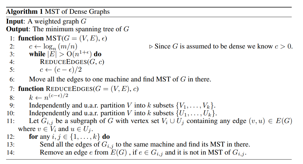
The main algorithm is the distributed MST algorithm (see below). Some notations:

$m$ is the number of edges $∣ E ∣$ , $n$ is the number of nodes $∣ V ∣$
$c$ measures the average density of the graph, i.e. the average number of edges per node. $l o g_{n} (m / n)$ is taken such that $c \in [0, 1]$ , where $c = 0$ implies that $∣ V ∣ = ∣ E ∣$ and $c = 1$ implies that $G$ is a fully connected graph.
$0 < ϵ < c$ is a density parameter controlling the final number of edges remaining before we run MST on a single machine. We can probably set it to $0.1$ or something like that. A higher $ϵ$ implies that we can run ReduceEdges for less steps, but we need more memory to run the final round of MST.


Distributed MST Algorithm

The algorithm is really quite simple. The main idea is that we can independently process each subgraph of $G$ comprising a random pair of vertex sets $V_{i} ⋃ U_{j}$ in a distributed fashion. Each worker finds the MST of the subgraph $G_{i, j}$ assigned to it, and any edge that is in $E (G_{i, j})$ but not in $MST (G_{i, j})$ may be removed from the global edge set $E (G)$ . In this way, we can whittle down the number of edges in $E (G)$ until it is a small set that can fit in memory (i.e. in the order of $O (n^{1 + ϵ})$ which is not much larger than the number of nodes). Then we can just run MST one final time on the master node.

So the algorithm really hinges on Lemma 6 in the paper, which tells us that removing edges in this distributed way will still give us the correct MST at the end.

Lemma 6. Let

G^{'} = (V^{'}, E^{'})

be a (not necessarily connected) subgraph of the input graph

G

. If an edge

e \in E^{'}

is not in the MST of

G^{'}

, then it is not in the MST of

G

either.

My proof by contradiction. Suppose an edge $e \in E (G)$ exists between nodes $A, B$ . Let $G^{'}$ denote a subgraph containing nodes $A, B$ , and suppose for contradiction that $e \in MST (G)$ but $e \in / MST (G^{'})$ .

First cut $MST (G)$ by removing the edge $e$ such that $A, B$ are in different partitions $P_{A}, P_{B}$ (each partition is a set of nodes). Observe that since $e$ exists in $MST (G)$ , it must be the lowest weight edge connecting $P_{A}$ and $P_{B}$ , since otherwise we could have replaced $e$ with a lower weight edge to complete the MST.

Now consider the subgraph $G^{'}$ and partition the nodes in $V^{'}$ according to $P_{A}, P_{B}$ to form $P_{A}^{'} \subset P_{A}$ and $P_{B}^{'} \subset P_{B}$ . Consider the MST of $G^{'}$ (might be a Minimum Spanning Forest instead, if not all nodes can be connected), and observe that there must exist a path between $A$ and $B$ in $G^{'}$ . Now remove any edges that cross $P_{A}^{'}$ and $P_{B}^{'}$ (call this edge set $E_{R}$ ). Then add back all the edges in $E_{R}$ that do not connect a path between nodes $A$ and $B$ .

Now there must exist exactly one edge remaining in $E_{R}$ that connects a path from $A$ to $B$ , since (i) a path exists between $A$ and $B$ in $G$ and (ii) there cannot be more than one edge that does so, otherwise there would have been a cycle in $MST (G^{'})$ . We also know that this edge is not $e$ .

But $e$ is the minimum weight edge between $P_{A}$ and $P_{B}$ , and therefore it must also be the minimum weight edge between $P_{A}^{'}$ and $P_{B}^{'}$ . Hence this other edge could not have been in the MST of $G^{'}$ . We reach a contradiction.

Thus we are justified in removing edges in this way. This lemma is great because it allows us to independently process each subgraph, and if memory is of concern, we can also batch the number of subgraphs processed at each step according to the number of workers we have.

Lastly, note that $c$ is a dynamic parameter in the algorithm that measures the density (i.e. number of edges relative to number of nodes) of the graph at each step. Since we reduce the density of the graph in every step, $c$ is stepped down progressively. This also results in $k$ being stepped down progressively, where $k$ controls the number of subgraphs at each step. We start with a large $k$ , which requires less memory since small subgraphs implies that many edges are "chopped off". As the graph becomes less dense, we can afford to lower $k$ progressively and remove more edges.

Implementation

I can't seem to find an implementation of this algorithm, but it is probably easy to write a naive version of it using multiprocessing in python. We could store the edges in a sqlite database and distribute a batch of subgraphs at each turn, collect the edges to remove in the master and remove them from the db, and repeat.

Chux's Notebook

Bateni 2017 - Affinity Clustering

Naive Algorithm

Efficient MST algorithm

Implementation