Lee 2022 - RQ-VAE

Autoregressive Image Generation using Residual Quantization

Vector quantization VQ-VAE is used to represent an image as a sequence of discrete codes. After quantizing, an autoregressive model (AR model, e.g. transformer) is used to predict the codes.

This paper aims to reduce the sequence length of the discrete codes, as it becomes more computationally efficient for the AR model. However, reducing the sequence length (aka reducing the spatial resolution) causes a rate-distortion trade-off. The dilemma is such:

• Increasing the codebook size improves resolution of discretization to preserve quality
• But increasing the codebook size also increases the probability of codebook collapse, where only a subset of codes are used

The main idea of RQ-VAE is to reduce the spatial resolution by more precisely approximating the feature map at each location. Instead of increasing the codebook size, we use the codebook to recursively quantize the feature map in a coarse-to-fine manner. That is, the feature representation at each location is the sum of the selected codebook vectors at each level. For a codebook where each level has $K$ codebook vectors and $D$ levels, we can represent $K^D$ vectors for learning just $D\times K$ vectors.

• The paper claims that due to this precise approximation, they can use just 8 x 8 latents to represent a 256 x 256 image. That is a reduction of 1024x!

Note: other papers usually use a distinct set of vectors for each codebook level, but in this paper they use a shared codebook for all levels. This is probably an implementation detail / hyperparameter to be tuned.

Method

There are two main stages:

• Stage 1: Residual Quantized VAE.
• Stage 2: RQ-Transformer.

Stage 1: Residual Quantized VAE

Let a codebook $\mathcal{C}$ be a finite set $\{(k,e(k))\},k\in [K]$ be a codebook of tuples of a code k and its code embedding $e(k)\in {\mathbb{R}}^{n_z}$.

• $K$ is the codebook size
• $n_z$ is the code embedding dimension

Given a vector $z\in {\mathbb{R}}^{n_z}$, let $Q(z;\mathcal{C})$ denote the discrete code of $z$: $$Q(z;\mathcal{C})=\underset{k\in [K]}{\mathrm{argmin}}||z-e(k)|{|}_2^2$$

The normal VQ-VAE flow is such:

• Start with an input image $X\in {\mathbb{R}}^{H_o\times W_o\times 3}$, where $H_o,W_o$ are the original image dimensions
• The encoder extracts a feature map $Z=\text{Enc}(X)\in {\mathbb{R}}^{H\times W\times n_z}$, where $H=H_o/f,W=W_o/f$ are downsampled $f$ times to form the latent feature map
• Applying the discretization independently to each position, we obtain a code map $M\in [K{]}^{H\times W}$: $$M_{h,w}=Q(Z_{h,w};\mathcal{C})$$
• We also obtain the quantized feature map $\hat{Z}\in {\mathbb{R}}^{H\times W\times n_z}$: $${\hat{Z}}_{h,w}=e(M_{h,w})$$
• Finally, we decode the quantized feature map to reconstruct the image: $$\hat{X}=G(\hat{Z})$$

For Residual Quantization, we instead represent $z\in {\mathbb{R}}^D$ as an ordered tuple of $D$ codes: $$RQ(z;\mathcal{C},D)=(k_1,...,k_D)\in [K{]}^D$$

Where $k_d$ is the discrete latent code of $z$ at depth $d$. Specifically, we obtain $k_d$ by recursively quantizing the residual. Starting with residual $r_o=z$, we compute the next $k_d,r_d$ as follows: $$\begin{array}{rl}{k}_d& =Q(r_{d-1};\mathcal{C})\\ r_d& =r_{d-1}-e(k_d)\end{array}$$

Finally, we represent $\hat{z}:={\hat{z}}^{(D)}={\sum }_{d=1}^{D}e(k_d)$ as the quantized embedding of $z$ using the sum of embedding across all depths.

Note: by using a shared codebook and summing up the embeddings at each depth, this resembles bloom hashing (see Weinberger 2009). The difference is that we recursively / sequentially encode the residuals, whereas bloom hashing simultaneously applies multiple independent hashes and sums up those embeddings at the hashed positions.

However, as the experiments indicate, the embedding norms get smaller as we go deeper into the codebook levels, since it learns a coarse-to-fine encoding. So it seems to make better sense to have separate codebook vectors for each level.

The RQ-VAE flow is thus identical to the VQ-VAE flow above, except that the discretization step differs:

• Start with an input image $X\in {\mathbb{R}}^{H_o\times W_o\times 3}$
• Encoder extracts $Z=\text{Enc}(X)\in {\mathbb{R}}^{H\times W\times n_z}$
• Discretize each position to get code map $M\in [K{]}^{H\times W\times D}$ (note the additional dimension $D$, since we now have $D$ codes per position): $$\begin{array}{rl}{M}_{h,w,d}& =RQ(Z_{h,w};\mathcal{C},d)\\ {\hat{Z}}_{h,w}& =\sum _{d=1}^{D}e(M_{h,w,d})\end{array}$$
• Finally decode: $\hat{X}=G(\hat{Z})$

RQ-VAE Training

The loss is: $$\begin{array}{rl}{\mathcal{L}}_{recon}& =||X-\hat{X}|{|}_2^2\\ {\mathcal{L}}_{commit}& =\sum _{d=1}^D||Z-\text{sg}[{\hat{Z}}^{(d)}]|{|}_2^2\\ \mathcal{L}& ={\mathcal{L}}_{recon}+\beta {\mathcal{L}}_{commit}\end{array}$$

The first loss is the reconstruction error of making the RQ-VAE roundtrip. The second loss is the commitment loss, which aims to push the encoder to reduce the quantization errors.

• Note that the commitment loss sums up the quantization error at each level of the codebook, not just the final quantization error at the end
• Also note that the authors did not include the loss to update the codebook as in VQ-VAE; instead they use the Exponential Moving Average approach to update the codebook $\mathcal{C}$ using the average encoder output assigned to each cluster

Stage 2: RQ-Transformer

Given that we have learned a code map of $M\in [K{]}^{H\times W\times D}$, the goal is to now autoregressively predict the code map (laid out in raster scan order). Specifically, let us lay out $M$ into a 2D array of codes $S\in [K{]}^{T\times D}$, where $T=H\times W$. Thus each row of $S$ (call it $S_t$) will contain $D$ codes: $$S_t=(S_{t1},...,S_{tD})\in [K{]}^D$$

Note that $S$ is laid out in raster scan order, meaning that we read the first row of pixels left-to-right, then move to the next row and so on.

Thus the goal of stage 2 is to learn an autoregressive model which learns the joint probability function $p(S)$, given all the prior tokens (i.e. causal masking). Note that we predict $D$ codes for each position before moving on to the next: $$p(S)=\prod _{t=1}^T\prod _{d=1}^{D}p(S_{td}|S_{<t},S_{t,<d})$$

The natural approach is to just fit an autoregressive transformer decoder to this unrolled sequence (of length $T\times D$, where $T=H\times W$). This incurs attention bottleneck complexity of $T^2{D}^2$. However, this paper argues that this is inefficient as it does not exploit the structure of our tokens, and proposes a customized RQ-transformer for this situation.

The idea is that there are two orthogonal dimensions, so we can decouple and create a specialized transformer to handle each one orthogonally:

• The first two dimensions, $H$ and $W$, encode the position
• The last dimension, $D$, encodes the depth

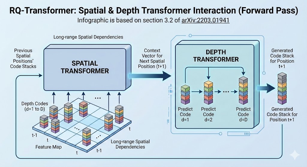RQ-Transformer Architecture

Spatial Transformer

The spatial transformer encodes the position dimension and marginalizes away the depth dimension. It is concerned with the "big picture". Specifically, each input position to the spatial transformer is: $$\begin{array}{rlr}{u}_t={\text{PE}}_T(t)+\sum _{d=1}^{D}e(S_{t-1},d)& & \text{ for }t>1\end{array}$$

Note that:

• ${\text{PE}}_T(t)$ is the position encoding for spatial position $t$
• We re-use the quantized embedding codebook vectors to represent inputs to the spatial transformer
• The depth position is marginalized out, such that we only need to encode $T=H\times W$ positions with the spatial transformer
• $u_1$ is a special case for start of sequence and will have its own learnable embedding

The sequence of inputs $(u_t{)}_{t=1}^T$ is passed into a causally masked transformer to produce spatial context vectors $h_t$ like so: $$h_t=\text{SpatialTransformer}(u_1,...,u_t)$$

Depth Transformer

Given the context vector $h_t$ provided by the spatial transformer, the depth transformer predicts a very short sequence of $D$ codes for this position $t$. Thus, the depth transformer can be a smaller stack of transformer layers.

• Note: in the experiments, generally $N_{spatial}=24$ and $N_{depth}=4$ in number of layers

Specifically, at spatial position $t$ and depth $d$, input $v_{t,d}$ to the depth transformer is the sum of codebook embeddings up to depth $d$: $$\begin{array}{rlrl}{v}_{t,d}& ={\text{PE}}_D(d)+h_t& & \text{ for }d=1\\ v_{t,d}& ={\text{PE}}_D(d)+\sum _{d^{\prime }=1}^{d-1}e(S_{t,d^{\prime }})& & \text{ for }d>1\end{array}$$

The short sequence of inputs $(v_{t1},...,v_{tD})$ is passed into a causally masked transformer + classifier head to predict the codes for each position. The same depth transformer is reused across all spatial positions $t$.

The autoregressive loss is simply the negative log likelihood of the correct latent token sequence: $${\mathcal{L}}_{AR}={\mathbb{E}}_S{\mathbb{E}}_{t,d}\left[-\log p(S_{t,d}|S_{<t},S_{t,<d})\right]$$

Computation Savings

As observed above, fitting a naive transformer to the full sequence of length $TD$ will incur attention complexity of $T^2{D}^2$. Compare this to the RQ-transformer:

• Spatial transformer: $T^2$, since we marginalize away the depth dimension
• Depth transformer: $T\times D^2$, since we re-use the depth transformer $T$ times
• RQ transformer: $T^2+T{D}^2$

With $T=512,D=4$, we have around 15x lower computational complexity:

• Naive approach: 4,194,304
• RQ transformer: 270,336
• Ratio: ~15x!

Other Tricks

There are two other tricks that they use in this paper, presumably to improve performance. The aim is to reduce the impact of exposure bias, which is the divergence between the samples during training and inference. During training, due to teacher forcing, we still get correct tokens to predict from at each position. During inference, since we generate each position autoregressively, errors can compound and lead the model to predict from a sequence that deviates far from what it has seen during training.

The main idea is to introduce some uncertainty into both the labels and inputs to the training process. Let us define a categorical distribution on $[K]$ conditioned by the encoder embedding $z\in {\mathbb{R}}^{n_z}$, with probability distribution: $$Q_{\tau }(k|z)\propto e^{-||z-e(k)|{|}_2^2/\tau }\text{ for }k\in [K]$$

Thus the probability of a discrete token $k$ increases exponentially as its quantized embedding $e(k)$ gets closer to the encoder embedding $z$. Note that as $\tau$ approaches $0$, $Q_{\tau }$ gets sharper and converges to the one-hot distribution $Q_0(k|z)=1[k=Q(z;\mathcal{C})]$.

This soft approximation of the argmin is used for soft labelling of the objective when training the RQ-transformer. Specifically, note that at position $t$ and depth $d$, we quantize by doing a nearest neighbour search for the residual vector $r_{t,d-1}$. Hence the hard target for the RQ-transformer training is the one-hot label $Q_0(\cdot |r_{t,d-1})$. Instead we replace with $Q_{\tau }(\cdot |r_{t,d-1})$.

We also do Stochastic Sampling of the latent codes when generating training samples for the RQ-transformer. Instead of deterministic code selection when encoding the raw images to latent codes, we sample from the categorical distribution of $Q_{\tau }(\cdot |r_{t,d-1})$.

The ablation studies show that using soft labelling + stochastic sampling significantly improves performance.

Results and Hyperparameters

General hyperparameters:

• Codebook size: $K=16,384$
• Codebook levels: $D=4$
• Latent dimension size: $n_z=256$
• Temperature: $\tau =0.5$

Generally RQ-VAE matches or outperforms image generation of other autoregressive competitors like VQ-GAN. It is also a lot faster in generation speed and memory usage.