Kaiser 2018 - Fast Decoding in Latent Space

Fast Decoding in Sequence Models using Discrete Latent Variables

This paper uses the idea in VQ-VAE to do fast decoding in latent space.

Main Idea

Transformers parallelize during training well, but are slow at inference due to autoregressive nature. This paper proposes to autoregressively generate in discrete latent space instead, which can be much faster depending on the compression:

• First auto-encode target sequence into discrete latent space which is a shorter sequence
• Train a decoder to generate in discrete latent space autoregressively
• Decode output sequence from the shorter latent sequence in parallel

Here is an infographic from nano banana that captures the idea of generation in latent space:

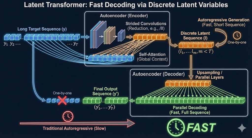Fast Generation in Latent Space

Setup

When generating sequential output, autoregressive models generates $y_1,...,y_n$ in a canonical order. This is because the model is trained to predict: $$P(y_t|y_{t-1},y_{t-2},...,y_1)$$

During training, because ground truth is known, we can train in parallel. During decoding, this is a fundamental limitation.

The proposal is to first encode the original sequence into a shorter sequence of discrete tokens $l_1,...,l_m$, where $m$ is much smaller than $n$. This latent sequence is also autoregressively predicted, and subsequently decoded in parallel back into the original token space. In the experiments, $m=\frac{n}{8}$.

Latent Transformer

The latent transformer is described in terms of a machine translation task. Given an input sequence $x$ in English, and a corresponding output sequence $y$ in German, our input-output pair is $(x,y)=(x_1,...,x_k,...,y_1,...,y_n)$.

The high level architecture is:

• The function $\text{ae}(y,x)$ will autoencode $y$ into a shorter sequence $l=l_1,...,l_m$ of discrete latent tokens using some discretization technique
• The latent prediction model $\text{lp}(x)$ which is a transformer will autoregressively predict $l$ based on $x$
• The decoder $\text{ad}(l,x)$ is a parallel model that will decode $y$ from $l$ and the input sequence $x$

Loss

The reconstruction loss compares the encoded - decoded output to the original target sequence $y$: $$\begin{array}{rl}\hat{y}& =\text{ad}(\text{ae}(y,x),x)\\ L_{recon}& =\text{CrossEntropyLoss}(\hat{y},y)\end{array}$$

The latent prediction loss compares the true latents generated by the autoencoder to the generated latents $\text{lp}(x)$: $$\begin{array}{rl}{l}_{true}& =\text{ae}(y,x)\\ l_{predicted}& =\text{lp}(x)\\ L_{latent}& =\text{CrossEntropyLoss}(l_{true},l_{predicted})\end{array}$$

The final loss is the sum of the two: $$L=L_{recon}+L_{latent}$$

Autoencoder

Now we describe each part in more detail. The diagram below summarizes the architecture of the autoencoder $\text{ae}(y,x)$.

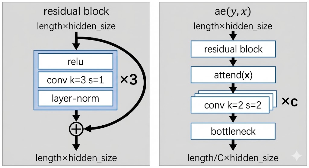Autoencoder architecture

The input to the autoencoder is of shape length x hidden_size. The aim is to shorten the sequence length by downsampling using convolutions.

We first pass through a residual block which aims to learn local features using convolutions:

• Pass through relu
• Pass through 1D convolution with k=3, s=1. This means we look over a window of 3 tokens each time, and take a step of 1 token each step.
  • Since stride is 1, the sequence length is unchanged
• Pass through layer norm + add the residual connection

Then we pass through a standard self attention block.

Then we pass c times through a downsampling convolution:

• k=2 means that we look over a window of 2 tokens
• s=2 means that we stride over 2 steps at a time: this effectively halves the sequene length
• Doing this c times means we get $C=2^c$ reduction in length

Finally we pass through the bottleneck function, which has yet to be described. But essentially the bottleneck function converts the representation of hidden_size at each position into a discrete token, and then represents it instead by the embedding of the discrete token using a lookup.

Decoder

The decoder $\text{ad}(l,x)$ decodes from latent space back into token space.

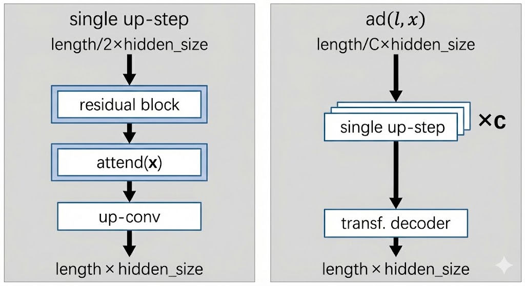Decoder architecture

We first pass through c up-steps, each of which will double the sequence length of the encoded sequence:

• The same residual block from before is used
• Self attention layer is used
• An up-conv step is performed:
  • A standard feed forward MLP is used that doubles the hidden dimension
  • A reshape operation is done to translate the extra hidden dimension into sequence length instead

Finally, the decompressed sequence of length x hidden_size is fed into a standard transformer decoder to decode the target sequence $y$.

• Note that for the first 10k steps of training, instead of feeding the decompressed sequence, the authors pretrain this decoder transformer model by feeding the target sequence $y$ (i.e. training it like a standard transformer decoder). This is to warm up the head so that gradients to upstream components are reasonable.

Discretization Bottleneck

This is actually the main part of the paper - how do we discretize our token sequence into latent space so that we can predict the latent tokens in an autoregressive manner?

The bottleneck function takes a target token embedding $y$ and maps it to a discrete token in $[K]:=\{1,2,...,K\}$:

• First, take $y$ and encode it: $\text{enc}(y)\in {\mathbb{R}}^D$, where $D$ is the dimension of the latent space.
• Next, pass the encoding through a bottleneck to product a discrete latent token $z_d(y)\in [K]$
• Look up embedding table using $z_d(y)$ to produce an embedding $z_q(y)\in {\mathbb{R}}^D$ to pass to the decoder

Note that the bottleneck function is applied to each sequence position in parallel, indepedently.

Gumbel Softmax

The gumbel-softmax trick is found in Jang 2016. It is a popular discretization technique.

First, we project the encoder output $\text{enc}(y)\in {\mathbb{R}}^D$ using a learned projection matrix $W\in {\mathbb{R}}^{K\times D}$, such that we get logits $l$: $$l=W\text{enc}(y)\in {\mathbb{R}}^K$$

We can simply extract the discrete code $z_d(y)$ for the decoder as: $$z_d(y)=\underset{i\in [K]}{\mathrm{argmax}}{l}_i$$

For evaluation and inference, we can simply use $j:=z_d(y)$ to look up an embedding table $e\in {\mathbb{R}}^{K\times D}$ to get $z_q(y)=e_j$. However, we cannot use this approach for training as the argmax and embedding lookup are non-differentiable.

For training, the Gumbel-softmax trick is used to make the whole thing differentiable.

• First, we draw $g_1,...,g_K\in \mathbb{R}$ i.i.d samples from the standard Gumbel distribution $$g_i\sim -\log (-\log u)\text{, where }u\sim \mathcal{U}(0,1)$$
• Then we compute the weight vector $w\in {\mathbb{R}}^K$ using a softmax, where for each latent dimension $i\in [K]$: $$w_i=\frac{\exp ((l_i+g_i)/\tau )}{{\sum }_{i=1}^K\exp ((l_i+g_i)/\tau )}$$
• Now we simply compute the input to the decoder as the weighted sum of the embedding table: $$z_q(y)=we\in {\mathbb{R}}^D$$

For low temperatures of $\tau$, $w$ would be close to representing the 1-hot arg-max index of $l$, which is what we use for evaluation and inference. Setting $\tau$ too high would cause divergence between training and inference, which is not ideal.

Why do we add the gumbel $g_i$? Ideally during training, we want the encoder logits $\text{Softmax}(l)$ to represent probabilities of a categorical distribution, from which we sample the discrete code $z_d(y)$. This ensures that we have:

• Exploration from the stochasticity
• Discretization. We also force the embedding $z_q(y)$ to be a single embedding (i.e. discretization) rather than a smooshed average of several embeddings.

The gumbel-max trick tells us that choosing $k=\mathrm{argmax}(l_i+g_i)$ results in an index $k$ distributed exactly according to $P(\text{class }k)$ as dictated by the softmax of the logits, which is what we want.

Since the gumbel-max is not differentiable, we simply relax it into a softmax operation, giving us the gumbel-softmax.

Vector Quantization

The VQ-VAE is covered in VQ-VAE. Here is a brief recap.

• The encoder output $\text{enc}(y)\in {\mathbb{R}}^D$ is used to do nearest neighbour lookup on embedding vectors $e\in {\mathbb{R}}^{K\times D}$ to give us:
  • $z_q(y)=e_k$ and $z_d(y)=k$
  • Where $k={\mathrm{argmin}}_{j\in [K]}||\text{enc}(y)-e_j|{|}_2$
• The loss is the reconstruction loss + the commitment loss between encoder output and codebook vectors: $$L=l_{recon}+\beta ||\text{enc}(y)-\text{sg}(z_q(y))|{|}_2$$

It turns out that the gradient update can be replaced by an exponential moving average over:

• The codebook embeddings $e_j$; and
• The count $c_j$ measuring the number of times $e_j$ is selected as a nearest neighbour

For a given mini-batch of target embeddings $\{y_1,...,y_l,...\}$, we can update the exponential moving average for counts like so: $$c_j\leftarrow \lambda c_j+(1-\lambda )\sum _{l}1[z_q(y_l)=e_j]$$

And the codebook embeddings $e_j$ updated as the average encoder output selected for $e_j$: $$e_j\leftarrow \lambda e_j+(1-\lambda )\sum _l\frac{1[z_q(y_l)=e_j]\text{enc}(y)}{c_j}$$

$\lambda$ is a decay parameter and set to $0.999$ in the experiments

Note. The paper also covers two other discretization techniques, namely improved semantic hashing and decomposed vector quantization (to counteract codebook collapse), but I don't cover it for now.

Results

The results show that the discretization bottleneck is not as good as a standard transformer, but beats all previous discrete methods and runs faster than a normal transformer.

Ablation results show that:

• Increasing the codebook size $K$ improves performance
• Increasing the ratio $n/m$ (i.e. shortening the sequence more aggressively) leads to speedup in inference but also clearly hurts performance

Hence it seems like there is no free lunch here.